pkgs <- c("fs", "futile.logger", "configr", "stringr", "ggpubr", "ggthemes",
          "jhtools", "glue", "ggsci", "patchwork", "tidyverse", "dplyr",
          "SummarizedExperiment", "jhuanglabRNAseq", "DESeq2", "maftools",
          "matrixStats", "Matrix", "furrr", "ComplexHeatmap")
for (pkg in pkgs){
  suppressPackageStartupMessages(library(pkg, character.only = T))
}

# load data info
merged_sinfo <- read_rds("~/projects/mm/docs/meta/sampleinfo/sampleinfo_jilin_commpass.rds")

# set color
config_fn <- "/cluster/home/ztao_jh/projects/mm/code/meta/check_new_cluster/checkin0250619/colors_fix.yaml"
config_list <- show_me_the_colors(config_fn, "all")
ig_colors <- config_list$Clinical_IgH

# load mutations
asian_mutations <- read_rds("/cluster/home/jhuang/projects/mm/analysis/meta/human/mutations/asian_mutations.rds")
cmps_mutations <- read_rds("/cluster/home/jhuang/projects/mm/analysis/meta/human/mutations/cmps_rna_wgs.rds")
jilin_mutations <- read_rds("/cluster/home/jhuang/projects/mm/analysis/meta/human/mutations/jilin_rna_wgs.rds")
bmc_hc_all <- read_rds("/cluster/home/yjliu_jh/projects/mm/output/data/hc_list.rds")

# data unify - cmps mutations
cmps_mutations$var <- cmps_mutations$EFFECT
cmps_mutations$var[cmps_mutations$var %in% c("frameshift_variant", "start_lost", "stop_gained", "stop_lost")] <- "frameshift"
cmps_mutations$var[cmps_mutations$var %in% c("inframe_deletion", "inframe_insertion")] <- "inframe"
cmps_mutations$var[cmps_mutations$var %in% c("splice_region_variant", "splice_donor_variant", "splice_acceptor_variant")] <- "splice"
cmps_mutations$var[cmps_mutations$var %in% c("missense_variant")] <- "missense"
cmps_mutations$var[cmps_mutations$var %in% c("synonymous_variant")] <- "Silent"
cmps_mutations$var[cmps_mutations$var %notin% c("Silent", "frameshift", "inframe", "splice", "missense")] <- "others"
cmps_mutations_fil <- cmps_mutations[cmps_mutations$Hugo_Symbol %in% keygenes, ]
cmps_mutations_fil <- cmps_mutations_fil[, c("sample_id", "Hugo_Symbol", "Chromosome", "Start_Position", "End_Position", "Tumor_Seq_Allele2", "var")] %>% distinct()

# data unify - bmc mutations
bmc_mutations <- bind_rows(bmc_hc_all, .id = "sample_id")
bmc_mutations$var <- as.character(bmc_mutations$Variant_Classification)
bmc_mutations$var[bmc_mutations$var %in% c("Frame_Shift_Del", "Frame_Shift_Ins", "Nonsense_Mutation", "Nonstop_Mutation")] <- "frameshift"
bmc_mutations$var[bmc_mutations$var %in% c("In_Frame_Ins", "In_Frame_Del")] <- "inframe"
bmc_mutations$var[bmc_mutations$var %in% c("Missense_Mutation")] <- "missense"
bmc_mutations$var[bmc_mutations$var %in% c("Splice_Region", "Splice_Site")] <- "splice"
bmc_mutations$var[bmc_mutations$var %notin% c("Silent", "frameshift", "inframe", "splice", "missense")] <- "others"

# data unify - jilin mutations
jilin_mutations$var <- as.character(jilin_mutations$Variant_Classification)
jilin_mutations$var[jilin_mutations$var %in% c("Frame_Shift_Del", "Frame_Shift_Ins", "Nonsense_Mutation", "Nonstop_Mutation")] <- "frameshift"
jilin_mutations$var[jilin_mutations$var %in% c("In_Frame_Ins", "In_Frame_Del")] <- "inframe"
jilin_mutations$var[jilin_mutations$var %in% c("Missense_Mutation")] <- "missense"
jilin_mutations$var[jilin_mutations$var %in% c("Splice_Region", "Splice_Site")] <- "splice"
jilin_mutations$var[jilin_mutations$var %notin% c("Silent", "frameshift", "inframe", "splice", "missense")] <- "others"

# data combine
asian_mutations2 <- rbind(bmc_mutations[, colnames(cmps_mutations_fil)], jilin_mutations[, colnames(cmps_mutations_fil)])
# mutations_all <- rbind(cmps_mutations_fil, asian_mutations2)

mutations_all <- rbind(unique(cmps_mutations[, colnames(cmps_mutations_fil)]), asian_mutations2)
mutations_all <- left_join(mutations_all, merged_sinfo[, c("sample_id", "ethnicity", "subtypes", "Clinical_IgH", "Dom_IgH_Type")])
mutations_all <- mutations_all[mutations_all$ethnicity %in% c("Asian", "Caucasian"), ]


# ------ mutation burden differences ------

mut_count_plot <- function (mut_dat, type_col, color) {
  type_name <- stringr::str_to_title(rlang::as_name(enquo(type_col)))
  mut_dat <- mut_dat %>% dplyr::filter(!is.na({{type_col}}))
  mut_count <- mut_dat %>%
    group_by(sample_id, {{type_col}}) %>%
    summarise(MutationCount = n(), .groups = "drop")
  subtype_order <- mut_count %>%
    group_by({{type_col}}) %>%
    summarise(MedianMut = median(MutationCount)) %>%
    arrange(desc(MedianMut)) %>%
    pull({{type_col}})
  mut_count <- mut_count %>%
    mutate(!!enquo(type_col) := factor({{type_col}}, levels = subtype_order)) %>%
    group_by({{type_col}}) %>%
    arrange(desc(MutationCount), .by_group = TRUE) %>%
    ungroup() %>%
    mutate(sample_id = factor(sample_id, levels = unique(sample_id)))
  mut_count <- mut_count %>%
    group_by({{type_col}}) %>%
    mutate(
      mid_idx = ceiling(n() / 2),
      x_label = if_else(row_number() == mid_idx, as.character({{type_col}}), "")
    ) %>% ungroup()

  p <- ggplot(mut_count, aes(x = sample_id, y = MutationCount, fill = {{type_col}})) +
    geom_bar(stat = "identity", width = 0.9) +
    scale_fill_manual(values = color) +
    theme_minimal() +
    theme(
      axis.text.x = element_text(angle = 45, hjust = 1),
      panel.grid.major.x = element_blank()
    ) +
    scale_x_discrete(labels = mut_count$x_label) +
    labs(
      x = glue::glue("{type_name} (each bar = one sample)"),
      y = "Mutation Count",
      fill = glue::glue("{type_name}"),
      title = glue::glue("Mutation Burden per Sample, Ordered by {type_name} Median")
    )
  return(p)
}


# test plots
testp <- mut_count_plot(mutations_all, subtypes, subtype_colors)
pdf("overall_test_mut_bar.pdf", height = 10, width = 15)
print(testp)
dev.off()21 Single Nucleotide Variations
Single Nucleotide Variations
21.1 SNVs from WGS
For the newly generated WGS dataset, single nucleotide variant (SNV) calling was performed using the germline mode of the DRAGEN platform. A stringent blacklist-based filtering pipeline was applied to ensure high specificity and consistency with existing publicly available data.
21.2 SNVs from RNAseq
Variant calling was performed using multiple tools followed by filtering steps based on allele frequency, depth, and strand bias. Samples with unusually low genome-wide coverage (<10× tumor, <5× normal), contamination, or evidence of sample mix-up were removed. Known common germline polymorphisms and SNVs with abnormally high freqency were filtered. SNVs with low VAF were removed.
21.3 SNVs from CoMMpass
For the CoMMpass public dataset, we adopted high-confidence WGS mutation calls from previously published studies and used these sites as a whitelist for filtering RNA-seq-based mutation calls. This strategy enhanced the credibility of mutation detection by minimizing methodological discrepancies (systematic biases), and facilitated alignment with prior research, enabling direct comparative analyses with existing studies.
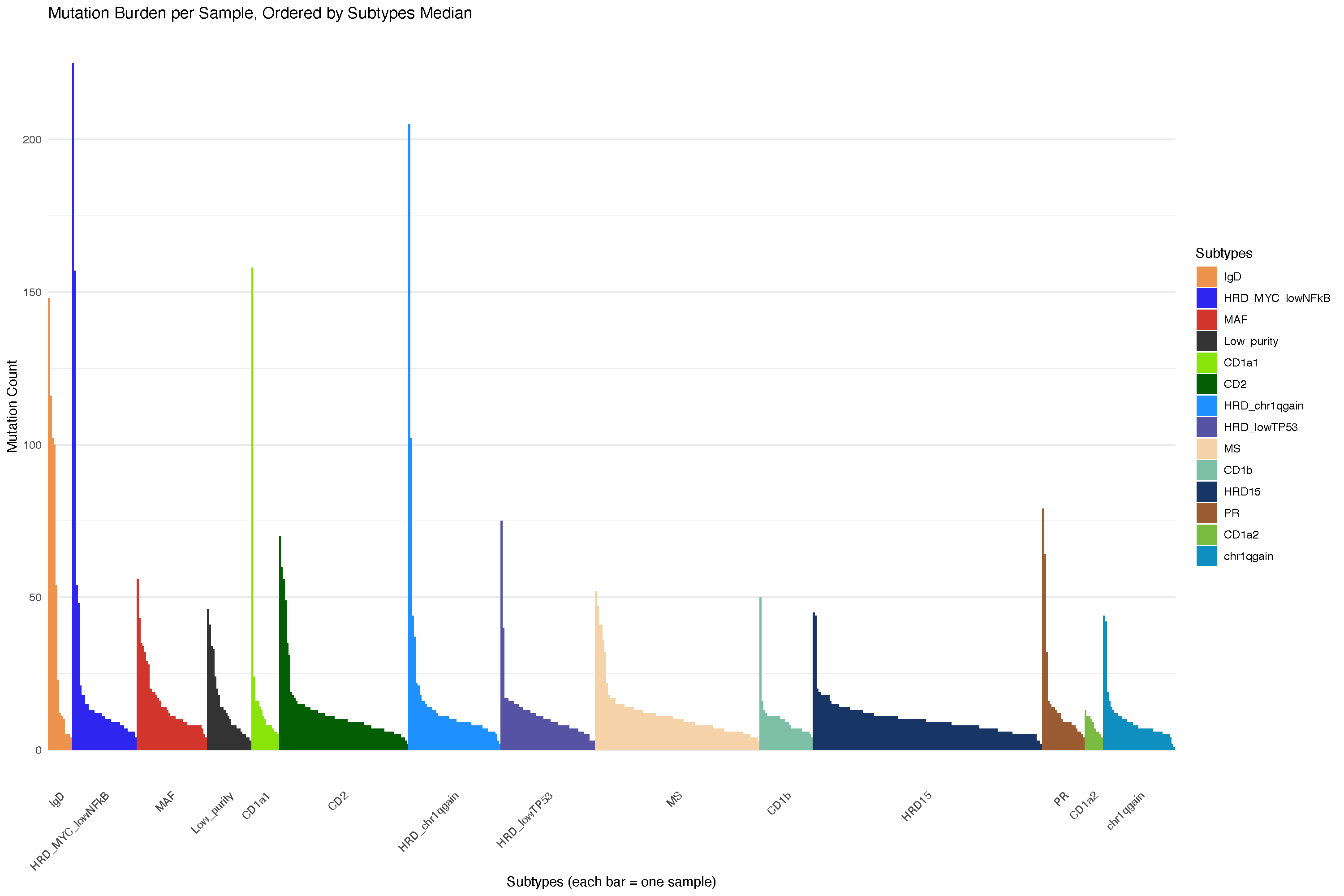
21.3.1 Mutation burden analysis
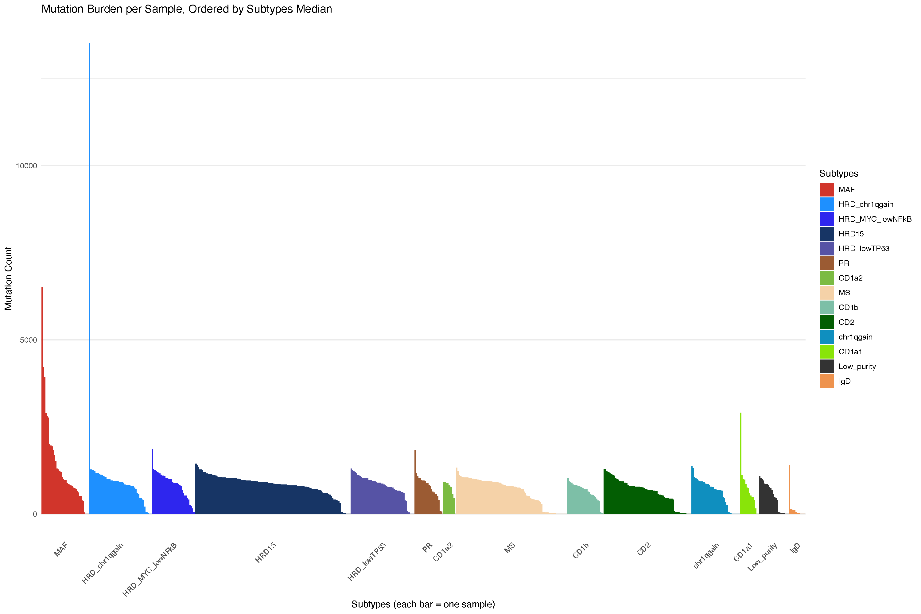
But that is unstable and may be affected by panel selection: