# Load necessary R packages for data processing and visualization
pkgs <- c("fs", "futile.logger", "configr", "ggpubr", "ggthemes", "jhtools",
          "glue", "ggsci", "patchwork", "tidyverse", "circlize", "ggrepel",
          "ComplexHeatmap", "GenomicRanges", "jhuanglabRNAseq", "ggh4x")
for (pkg in pkgs){
  suppressPackageStartupMessages(library(pkg, character.only = T))
}

# Define project parameters
project <- "mm"
dataset <- "meta"
species <- "human"
workdir <- glue("~/projects/{project}/output/{dataset}/{species}/figures/fig1") |> checkdir()
setwd(workdir)31 Figure 1
31.1 Figure 1
31.2 Setup
Load required R packages and set the working directory.
31.3 enrich score of public gene sets in MM subtypes
# read in data
objht <- read_rds("/cluster/home/jhuang/projects/mm/analysis/meta/human/rnaseq/figures/heatmap/step1/heatmap_0.9_groups16.rds")
df <- read_rds("/cluster/home/jhuang/projects/mm/docs/meta/sampleinfo/sampleinfo_jilin_commpass.rds")
config_fn <- "~/projects/mm/output/meta/human/figures/colors_fix.yaml"
config_list <- show_me_the_colors(config_fn, "all")

subdf <- tibble(sample_id = rownames(objht$heatmap2[[6]])) |>
  left_join(df) |>
  mutate(
    treatment_group = case_when(treatment_group %in% "Unknown" ~ NA_character_,
                                T ~ treatment_group),
    hit_event = str_extract(hit_event, pattern = "\\d+"),
    best_response = case_when(
      best_response == "SCR" ~ "sCR",
      best_response == "≥VGPR" ~ "VGPR",
      best_response == "Unknown" ~ NA_character_,
      T ~ best_response
    )
  )

out_dir <- dir_create("./score_dotplot/")
all_scores <- c("subtypes", config_list$paper_scores)
subdf_score <- subdf[,all_scores]
subdf_score[,config_list$paper_scores] <- apply(subdf_score[,config_list$paper_scores], 2, function(x){
  (x-min(x))/(max(x) - min(x))
  # scale(x)
})
subdf_score$subtypes = factor(subdf_score$subtypes, levels = rev(unique(subdf_score$subtypes)))

dotplotdf <- subdf_score |>
  pivot_longer(- subtypes) |>
  group_by(subtypes, name) |>
  summarise(
    positive_rate = sum(value > 0.5)/n(),
    mean_score = mean(value)) |>
  ungroup() |>
  mutate(name = factor(name, levels = config_list$paper_scores))

score_dotplot <- ggplot(dotplotdf |> mutate(label = str_extract(name, pattern = ".+?et_al")),
       aes(x = name, y = subtypes, fill = mean_score, size = positive_rate)) +
  geom_point(shape = 21)+
  scale_fill_gradientn(limits = c(0.1, 0.9),
                       colours = c("#1E90FF", "white","#DC143C"),
                       values = scales::rescale(c(0.1, 0.5, 0.9)),
                       oob = scales::squish,
                       name = "Z-Score")+
  theme_few() +
  facet_grid(1~ label, scales = "free_x", space = "free_x") +
  theme(axis.text.x = element_text(angle = 45, hjust = 1, vjust = 1),
        axis.title.x = element_blank(),
        # axis.text.y = element_blank(),
        axis.ticks.length.y = unit(0, "mm"),
        axis.ticks.length.x = unit(0, "mm"),
        legend.position = "right",
        panel.spacing = unit(-1, "mm"),
        strip.text.y.right = element_blank(),
        strip.text.x.top = element_blank(),
        strip.background = element_rect(fill = NA),
        # plot.margin = margin(l = 1),
        panel.border = element_rect(fill = NA, color = "black", size = 0.5))
pdf(glue("{out_dir}/score_dotplot.pdf"), width = 12, height = 5)
print(score_dotplot)
dev.off()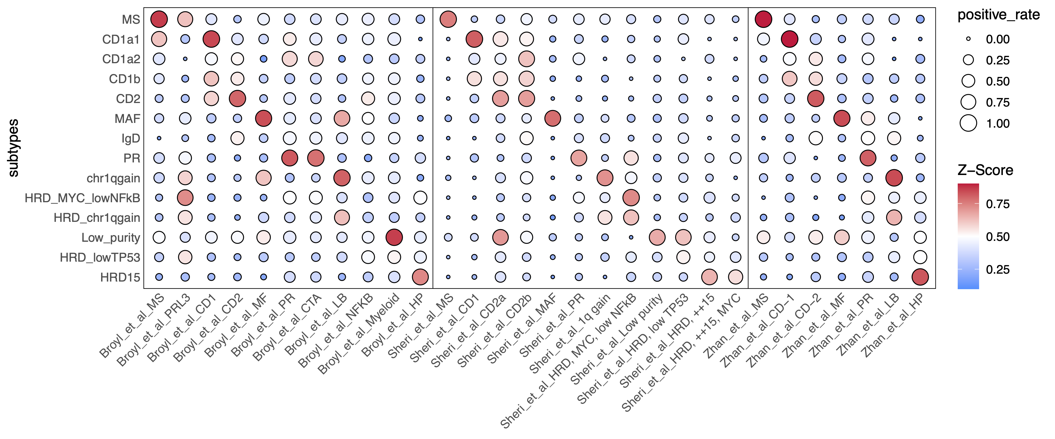
31.4 Refined molecular subtypes of MM
# colors settings
col <- config_list[c("gender", "ethnicity", "age", "GEP70", "Clinical_IgH", "Clinical_IgL", "batch", "subtypes", "imwg_risk",
                     "treatment_group", "best_response", "hit_event")]
col$ethnicity <- c(col$ethnicity, "other" = "grey")
col$datasets <- config_list$batch
col$GEP70 <- colorRamp2(quantile(subdf$GEP70, c(0.1, 0.5, 0.9), na.rm = TRUE),
                        colors = col$GEP70[c("colors1", "colors2", "colors3")])
col$age <- colorRamp2(quantile(subdf$age, as.numeric(col$age[c("breaks1", "breaks2", "breaks3")]), na.rm = TRUE),
                      colors = col$age[c("colors1", "colors2", "colors3")])

out_dir <- dir_create("./cluster_heatmap/")

# draw
all_col <- config_list$clinical_order
show_legend <- config_list$show_legend

hasub2 <- HeatmapAnnotation(df = subdf[,all_col],
                            annotation_name_side = "left",
                            show_legend = all_col %in% show_legend,
                            col = col)

ht <- Heatmap(t(objht$heatmap2[[6]]),
              show_column_names = FALSE,
              show_row_names = FALSE,
              top_annotation = hasub2,
              name = "Z-Score",
              border = TRUE,
              cluster_columns = FALSE,
              cluster_rows = FALSE,
              column_gap = unit(0, "mm"),
              column_title_rot = 90,
              clustering_method_columns = "ward.D2",
              clustering_method_rows = "ward.D2",
              heatmap_width = unit(160, "mm"),
              column_split = as.numeric(factor(subdf$subtypes, levels = unique(subdf$subtypes))),
              column_title = unique(subdf$subtypes))

pdf(glue("{out_dir}/figure1_heatmap.pdf"), width = 14, height = 6)
draw(ht, annotation_legend_side = "right", heatmap_legend_side = "left")
dev.off()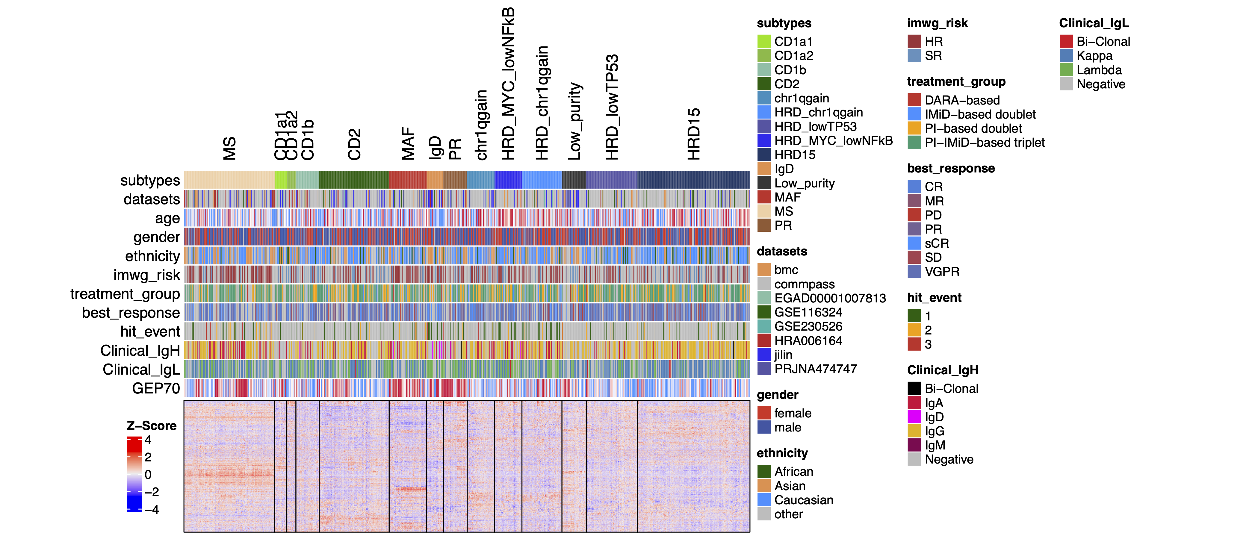
31.5 TSNE of subtypes
out_dir <- dir_create("./tsne/")
mm_heatmap <- "/cluster/home/jhuang/projects/mm/analysis/meta/human/rnaseq/exp/mm_heatmap1117.rds" %>%
  read_rds() |> convert_df_plot()
dat_exp <- mm_heatmap[colnames(objht$heatmap2[[6]]), ] |> t()

pca_raw <- prcomp(dat_exp, scale. = TRUE)
pca_mat <- as.data.frame(pca_raw$x[, 1:2])
tsne_raw <- Rtsne::Rtsne(dat_exp, perplexity = 30, max_iter = 1000,
                         verbose = FALSE, check_duplicates = FALSE)
tsne_mat <- as.data.frame(tsne_raw$Y)
colnames(tsne_mat) <- c("tSNE_1", "tSNE_2")
rownames(tsne_mat) <- rownames(dat_exp)
tsne_mat$sample_id <- rownames(tsne_mat)
tsne_mat <- tsne_mat |>
  left_join(
    subdf[,c("sample_id", "subtypes", "datasets", "ethnicity", "Clinical_IgH")] |>
      mutate(
        datasets = factor(datasets, levels = c("HRA006164", "jilin", "PRJNA474747", "bmc", "GSE116324", "GSE230526", "EGAD00001007813", "commpass")),
        ethnicity = factor(ethnicity, levels = c("Asian", "African", "Caucasian", "other")),
        Clinical_IgH = factor(Clinical_IgH, levels = c("IgM", "Bi-Clonal", "IgD", "IgA", "IgG", "Negative")),
      )
  )


pdf(glue("{out_dir}/embedding_plot.pdf"), width = 7, height = 6)
ggplot(tsne_mat,
       aes(x = tSNE_1, y = tSNE_2, color = subtypes)) +
  geom_point() +
  ggrepel::geom_label_repel(data = tsne_mat |>
               group_by(subtypes) |>
               summarise(tSNE_1 = mean(tSNE_1),
                         tSNE_2 = mean(tSNE_2)),
             mapping = aes(x = tSNE_1, y = tSNE_2, label = subtypes, fill = subtypes), color = "white") +
  scale_color_manual(values = col$subtypes) +
  scale_fill_manual(values = col$subtypes) +
  theme_void() +
  theme(legend.position = "none")
dev.off()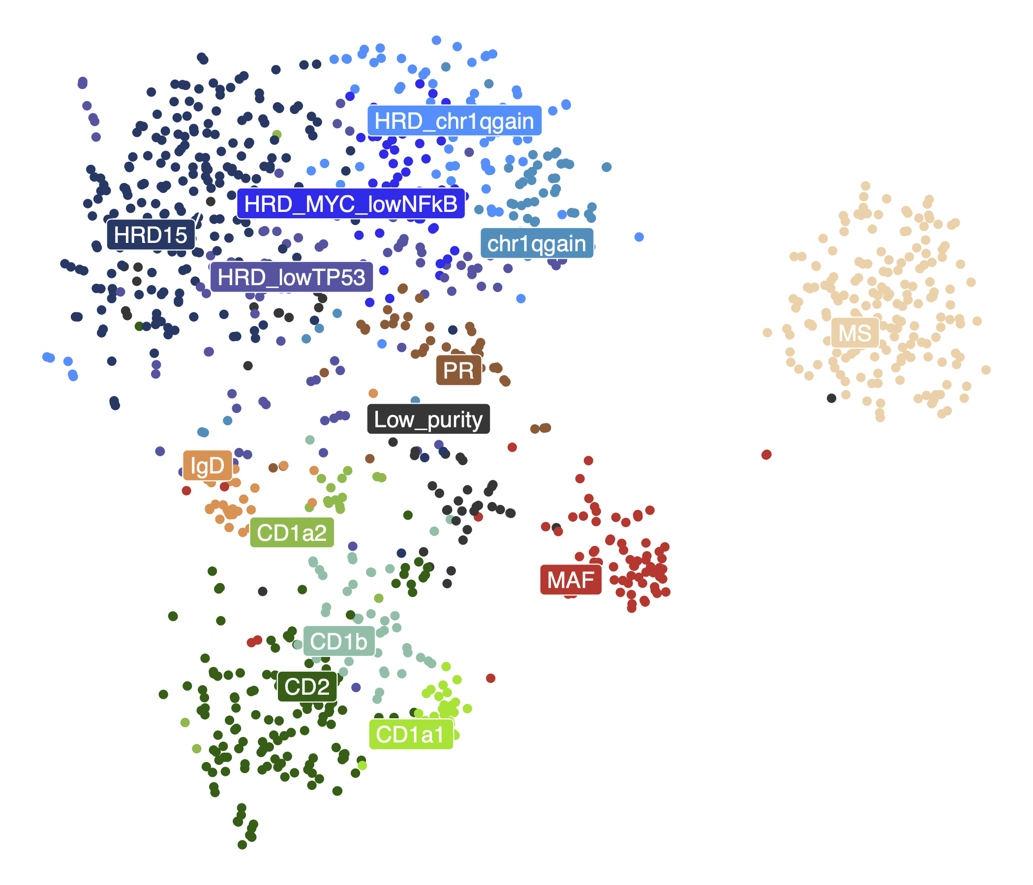
31.5.1 clinical features of subtypes
code: