pkgs <- c("fs", "futile.logger", "configr", "stringr", "ggpubr", "ggthemes",
          "jhtools", "glue", "ggsci", "patchwork", "tidyverse", "dplyr",
          "SummarizedExperiment", "jhuanglabRNAseq", "DESeq2", "maftools",
          "matrixStats", "Matrix", "furrr", "ComplexHeatmap", "rstatix",
          "clusterProfiler", "DOSE", "enrichplot", "org.Hs.eg.db",
          "EnhancedVolcano")
for (pkg in pkgs){
  suppressPackageStartupMessages(library(pkg, character.only = T))
}

#
setwd("/cluster/home/yjliu_jh/projects/mm/output/relapse_paired")
salmon_dir <- "/cluster/home/jhuang/projects/mm/analysis/EGAD00001007813/human/rnaseq/salmon"
samples <- list.files(salmon_dir)
patients <- sub("_.*", "", samples)
paired_patients <- patients[duplicated(patients)]
all_paired_samples <- c(paste0(paired_patients, "_Diagnosis"), paste0(paired_patients, "_Relapse1"))19 Differentially Expressed Genes
Differentially Expressed Genes
19.1 Differential Expression Analysis Workflow and Rationale
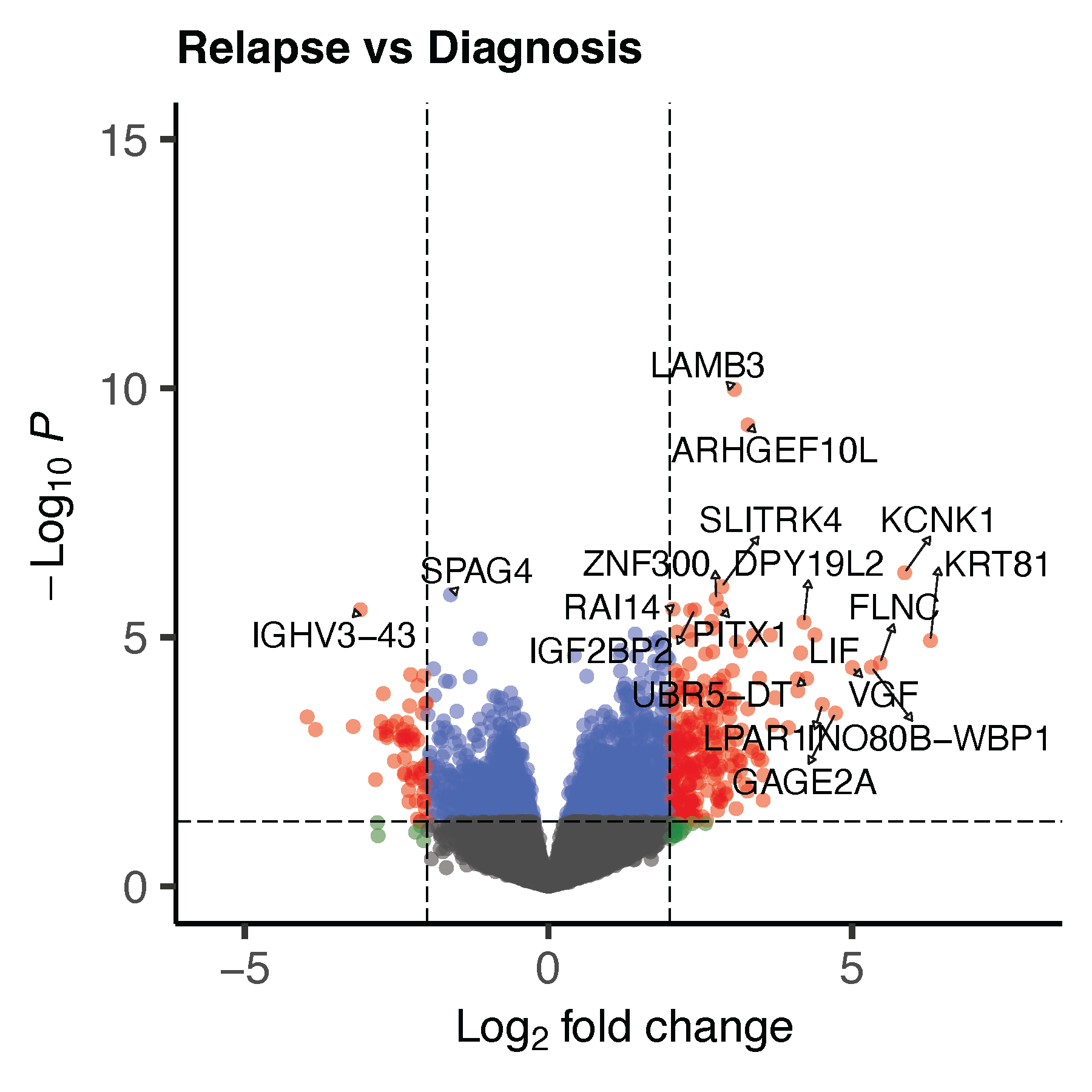
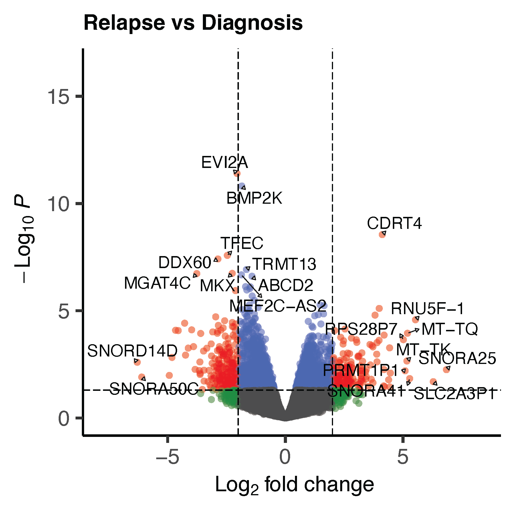
To identify genes that are differentially expressed between specified sample groups, we performed differential expression analysis using the DESeq2 R package (v1.46.0). The DESeq2 framework models count-based RNA-seq data using negative binomial distributions, which are well-suited for capturing the discrete and overdispersed nature of RNA-seq count data. Unlike methods that rely on normalized or transformed expression values, DESeq2 operates directly on raw, unnormalized counts, allowing for the modeling of biological and technical variability through shrinkage estimation and empirical Bayes approaches. One key strength of DESeq2 lies in its ability to estimate dispersion parameters for each gene across samples while borrowing information across all genes to stabilize variance estimates—particularly valuable for genes with low or moderate counts. Additionally, DESeq2 includes procedures for normalization based on size factors, which account for differences in sequencing depth and RNA composition between samples. These model-based adjustments make the method robust to both library size variation and global expression shifts. Statistical significance for differential expression was assessed using Wald tests, and p-values were adjusted for multiple hypothesis testing using the Benjamini–Hochberg false discovery rate (FDR) procedure. In this paper, genes with adjusted p-values < 0.01 and absolute log₂ fold changes exceeding 1.5 were considered significantly differentially expressed, which is colored differently in the volcano plots.
19.2 Use of Variance-Stabilizing Transformation (VST)
In addition to DE analysis, we applied the variance stabilizing transformation (VST) implemented in DESeq2 to obtain expression matrices suitable for downstream multivariate analyses, such as principal component analysis (PCA), batch effect correction, and clustering. The VST transforms raw counts to a log-like scale that approximately stabilizes the variance across the full dynamic range of expression, while preserving the relative ordering of gene expression levels. Compared to simple log₂(count + 1) transformations, VST more effectively reduces the influence of high-count genes and avoids over-amplifying noise in low-count genes, especially in datasets with substantial expression range heterogeneity.
19.3 Application in Cross-dataset Integration
When integrating gene expression data from multiple cohorts or datasets, technical differences such as sequencing depth, platform, and library preparation protocols can introduce significant batch effects. VST-transformed data are advantageous in such settings because the transformation partially normalizes for sequencing depth and heteroscedasticity, allowing for more reliable cross-dataset comparison of gene expression patterns. In our study, VST was applied to each dataset independently after normalization, followed by appropriate batch correction (the ComBat algorithm) prior to unsupervised clustering and subtype classification. The use of VST ensured that expression variation was not dominated by technical artifacts, and that biologically meaningful signals were preserved across datasets.
19.4 Differential Expression Analysis Strategy
Differential expression analysis was performed across multiple comparison contexts, including between MM subtypes, between different disease states (e.g., baseline vs. relapse), and between MM samples and normal plasma cells. When paired samples were available (e.g., pre- and post-relapse from the same patient), a paired design was employed to account for inter-individual variability. In all other comparisons, unpaired designs were used. Technical variables such as sequencing method (mRNA-seq vs. total RNA-seq) and dataset of origin were included as covariates to adjust for potential batch effects. Below is an example workflow of the DE analysis:
Set up and sample preparation:
Define sequencing types based on uncorrected data
mmdatasets <- c("jilin", "commpass", "public", "HRA005897")
count_files <- glue::glue("/cluster/home/jhuang/projects/mm/analysis/{mmdatasets}/human/rnaseq/exp/tables/{mmdatasets}_human_counts.csv")
total_counts_list <- lapply(count_files[file.exists(count_files)], read_csv)
names <- mmdatasets[file.exists(count_files)]
counts_all <- total_counts_list[[1]]
for (i in 2:length(total_counts_list)) {
  counts_all <- bind_cols(counts_all, total_counts_list[[i]][, -(1:2)])
}
hugo_anno <- readr::read_delim("/cluster/home/yjliu_jh/projects/mm/data/hgnc_complete_set.txt",
                               col_types = cols(intermediate_filament_db = col_character()))
hugo_anno <- hugo_anno[, c("symbol", "ensembl_gene_id", "locus_group")] %>% as.data.frame()
colnames(hugo_anno)[2] <- "gene_id"

# prepare counts data
counts_all <- counts_all[, -2] %>% left_join(hugo_anno) %>% na.omit() %>%
  dplyr::select(-c(gene_id, locus_group)) %>% as.data.frame() %>% remove_rownames() %>%
  column_to_rownames(var = "symbol") %>% as.matrix() %>% round()

# get exp
pred_rna_lib <- function (dat_mat) {
  typical_genes <- c("H4C3", "H4C4", "RN7SL1")
  inter_genes <- intersect(typical_genes, rownames(dat_mat))
  stopifnot("please make sure enough genes is contained in the data" = length(inter_genes) > 0)
  dat_mat <- log(dat_mat[rownames(dat_mat) %in% inter_genes, ] + 1)
  clust <- data.frame(cluster = cutree(hclust(dist(t(dat_mat))), k = 2))
  diff <- mean(unlist(dat_mat[, clust$cluster %in% 1])) - mean(unlist(dat_mat[, clust$cluster %in% 2]))
  clust$rna_type <- "mRNA"
  clust$rna_type[clust$cluster == (2 - sum(diff > 0))] <- "total_RNA"
  new_dat <- data.frame(sample_id = rownames(clust), rna_type = clust$rna_type)
  return(new_dat)
}

rna_lib_large <- pred_rna_lib(counts_all)
readr::write_rds(rna_lib_large, "/cluster/home/yjliu_jh/projects/mm/output/rna_lib_mm_samples.rds")
Perform paired DE analysis on the first set:
counts_mm <- read_csv("/cluster/home/jhuang/projects/mm/analysis/EGAD00001007813/human/rnaseq/exp/tables/EGAD00001007813_human_counts.csv")
new_counts <- counts_mm[, -2] %>% left_join(hugo_anno) %>% na.omit() %>%
  dplyr::select(-c(gene_id, locus_group)) %>% as.data.frame() %>% remove_rownames() %>%
  column_to_rownames(var = "symbol") %>% as.matrix() %>% round()
new_counts <- new_counts[, all_paired_samples]
ega_si1 <- data.frame(patient_id = rep(paired_patients, 2),
                      sample_id = all_paired_samples,
                      type = rep(c("Diagnosis", "Relapse"), each = length(paired_patients)))
dds <- DESeqDataSetFromMatrix(new_counts, ega_si1, ~ patient_id + type)
keep <- rowSums(counts(dds) >= 5) > ceiling(0.2 * ncol(dds))   ## if no filter, many with embryonic morphogenesis. Oncofetal reprogramming?
dds <- dds[keep, ]
keep2 <- rowSums(counts(dds) == 0) < ceiling(0.5 * ncol(dds))
dds <- dds[keep2, ]
dds <- DESeq(dds)
Helper functions:
add_col <- function(data){
  data$gene_name <- rownames(data)
  data$absFC <- abs(data$log2FoldChange)
  data <- data[order(data$pvalue), ]
  data2 <- left_join(as.data.frame(data), hugo_anno[, c("symbol", "gene_id")], by = c("gene_name" = "symbol"))
  data$ensembl_id <- data2$gene_id
  data
}

quick_volcano <- function (resA, title, k = 7) {
  p <- EnhancedVolcano(resA,
                       lab = resA$gene_name,
                       title = title,
                       subtitle = NULL,
                       caption = NULL,
                       legendPosition = "none",
                       selectLab = unique(c(resA[order(resA$padj), ][1:10, k],
                                            resA[order(resA$absFC, decreasing = T), ][1:10, k])),
                       drawConnectors = TRUE,
                       #min.segment.length = 1,
                       widthConnectors = 0.3,
                       x = 'log2FoldChange',
                       y = 'pvalue',
                       pCutoff = 0.05,
                       FCcutoff = 2.0,
                       gridlines.major = FALSE,
                       gridlines.minor = FALSE)
  p
}
Get DE results and perform basic functional enrichment:
res_ega1 <- add_col(results(dds, c("type", "Relapse", "Diagnosis")))
GSEAInput_a <- data.frame(rownames(res_ega1), res_ega1$log2FoldChange)
colnames(GSEAInput_a) <- c("Symbol", "logFC")
GSEA2 <- GSEAInput_a$logFC
names(GSEA2) <- as.character(GSEAInput_a$Symbol)
GSEA2 <- sort(GSEA2, decreasing = TRUE)
gseGO_res_a <- gseGO(GSEA2, OrgDb = org.Hs.eg.db, keyType = "SYMBOL", ont = "BP",
                     minGSSize = 5, maxGSSize = 1000, pvalueCutoff = 0.2)
Perform similar analysis on the Jilin dataset:
merged_sinfo <- read_rds("~/projects/mm/docs/meta/sampleinfo/sampleinfo_jilin_commpass.rds")

# in our data
counts_jilin <- read_csv("/cluster/home/jhuang/projects/mm/analysis/jilin/human/rnaseq/exp/tables/jilin_human_counts.csv")
counts_jilin <- counts_jilin[, -2] %>% left_join(hugo_anno) %>% na.omit() %>%
  dplyr::select(-c(gene_id, locus_group)) %>% as.data.frame() %>% remove_rownames() %>%
  column_to_rownames(var = "symbol") %>% as.matrix() %>% round()
sinfo_jilin <- merged_sinfo[merged_sinfo$sample_id %in% colnames(counts_jilin), c("sample_id", "cn_name", "tumor_descriptor")] %>% unique()
sinfo_jilin2 <- sinfo_jilin[sinfo_jilin$tumor_descriptor %notin% "initial_treating", ]
temp_count <- sinfo_jilin2 %>% group_by(cn_name) %>% summarise(c = length(unique(tumor_descriptor)))
temp_patients <- temp_count$cn_name[temp_count$c > 1]
sinfo_jilin2 <- sinfo_jilin2[sinfo_jilin2$cn_name %in% temp_patients, ]
sinfo_jilin2 <- sinfo_jilin2[!duplicated(sinfo_jilin2[, 2:3]), ] %>% as.data.frame()
sinfo_jilin2 <- sinfo_jilin2[order(sinfo_jilin2$cn_name, sinfo_jilin2$tumor_descriptor), ]
rownames(sinfo_jilin2) <- sinfo_jilin2$sample_id
counts_jilin_paired <- counts_jilin[, rownames(sinfo_jilin2)]

dds <- DESeqDataSetFromMatrix(counts_jilin_paired, sinfo_jilin2, ~ cn_name + tumor_descriptor)
keep <- rowSums(counts(dds) >= 5) > ceiling(0.2 * ncol(dds))
dds <- dds[keep, ]
keep2 <- rowSums(counts(dds) == 0) < ceiling(0.5 * ncol(dds))
dds <- dds[keep2, ]
dds <- DESeq(dds)

res_jilin2 <- add_col(results(dds, c("tumor_descriptor", "Recurrence", "Primary")))
GSEAInput_c <- data.frame(rownames(res_jilin2), res_jilin2$log2FoldChange)
colnames(GSEAInput_c) <- c("Symbol", "logFC")
GSEA2 <- GSEAInput_c$logFC
names(GSEA2) <- as.character(GSEAInput_c$Symbol)
GSEA2 <- sort(GSEA2, decreasing = TRUE)
gseGO_res_c <- gseGO(GSEA2, OrgDb = org.Hs.eg.db, keyType = "SYMBOL", ont = "BP",
                     minGSSize = 5, maxGSSize = 1000, pvalueCutoff = 0.2)
Plots representing DE results:
volcano_p <- quick_volcano(as.data.frame(res_ega1), "Relapse vs Diagnosis")
ggsave("volcano_ega1.pdf", volcano_p, dpi = 300, width = 6, height = 6, units = "in")
res_a <- as.data.frame(gseGO_res_a)
res_a$regulation <- ifelse(res_a$NES > 0, "activated", "suppressed")
res_a <- res_a[, c(1:2, 12, 3:11)]
pdf("Relapse_vs_Diagnosis.pdf", width = 12, height = 9)
print(dotplot(gseGO_res_a, showCategory = 9, split = ".sign") + facet_grid(.~.sign))
dev.off()

volcano_p <- quick_volcano(as.data.frame(res_jilin2), "Relapse vs Diagnosis")
ggsave("volcano_jilin_paired.pdf", volcano_p, dpi = 300, width = 6, height = 6, units = "in")
pdf("Relapse_vs_Diagnosis_jilin_paired.pdf", width = 12, height = 9)
print(dotplot(gseGO_res_c, showCategory = 9, split = ".sign") + facet_grid(.~.sign))
dev.off()
19.5 Volcano plots:
Paired plot showing expression changes:
# pair plot of relapse-primary samples
pair_plot2 <- function(data, gene, anno){

  gene_pair <- data.frame(sample_id = names(data[rownames(data) %in% gene, ]),
                          exp = as.numeric(data[rownames(data) %in% gene, ]))
  gene_pair <- left_join(gene_pair, anno)

  p1 <- ggplot(gene_pair, aes(class, exp, fill = class))+
    geom_line(aes(group = patient_id), size = 1) +
    geom_point(shape = 21, size = 3, stroke = 0.6, color = 'black')+
    scale_x_discrete(expand = c(-1.05, 0)) +
    scale_fill_manual(values = c("#FC6666", "#108080"))+
    geom_rangeframe() +
    theme_tufte() +
    theme(legend.position = 'none',
          axis.text.y = element_text(size = 14, face = "bold"),
          axis.text.x = element_text(size = 12, face = "bold"),
          axis.title.y = element_text(size = 15, color = "black", face = "bold"),
          axis.title.x = element_text(size = 15, color = "black", face = "bold")) +
    labs(x = gene, y = 'Values')
  p1

}

exp_ega1 <- assay(vst(dds))
ega_si1 <- data.frame(patient_id = sub("_.*", "", colnames(exp_ega1)),
                      sample_id = colnames(exp_ega1),
                      class = rep(c("Diagnosis", "Relapse"), each = ncol(exp_ega1) * 0.5))

testp_LAMB3 <- pair_plot2(exp_ega1, "LAMB3", ega_si1)
pdf("test_pair_LAMB3.pdf", height = 5, width = 3)
print(testp_LAMB3 + coord_cartesian(xlim = c(1, 2.2)))
dev.off()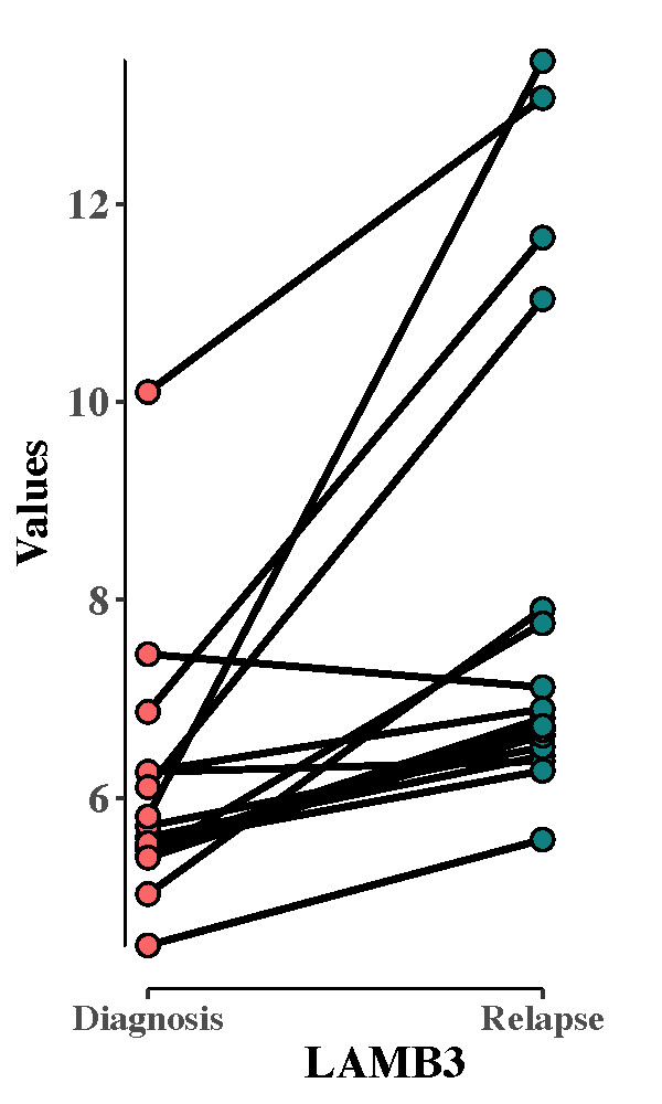
Dotplots showing functional enrichment results:
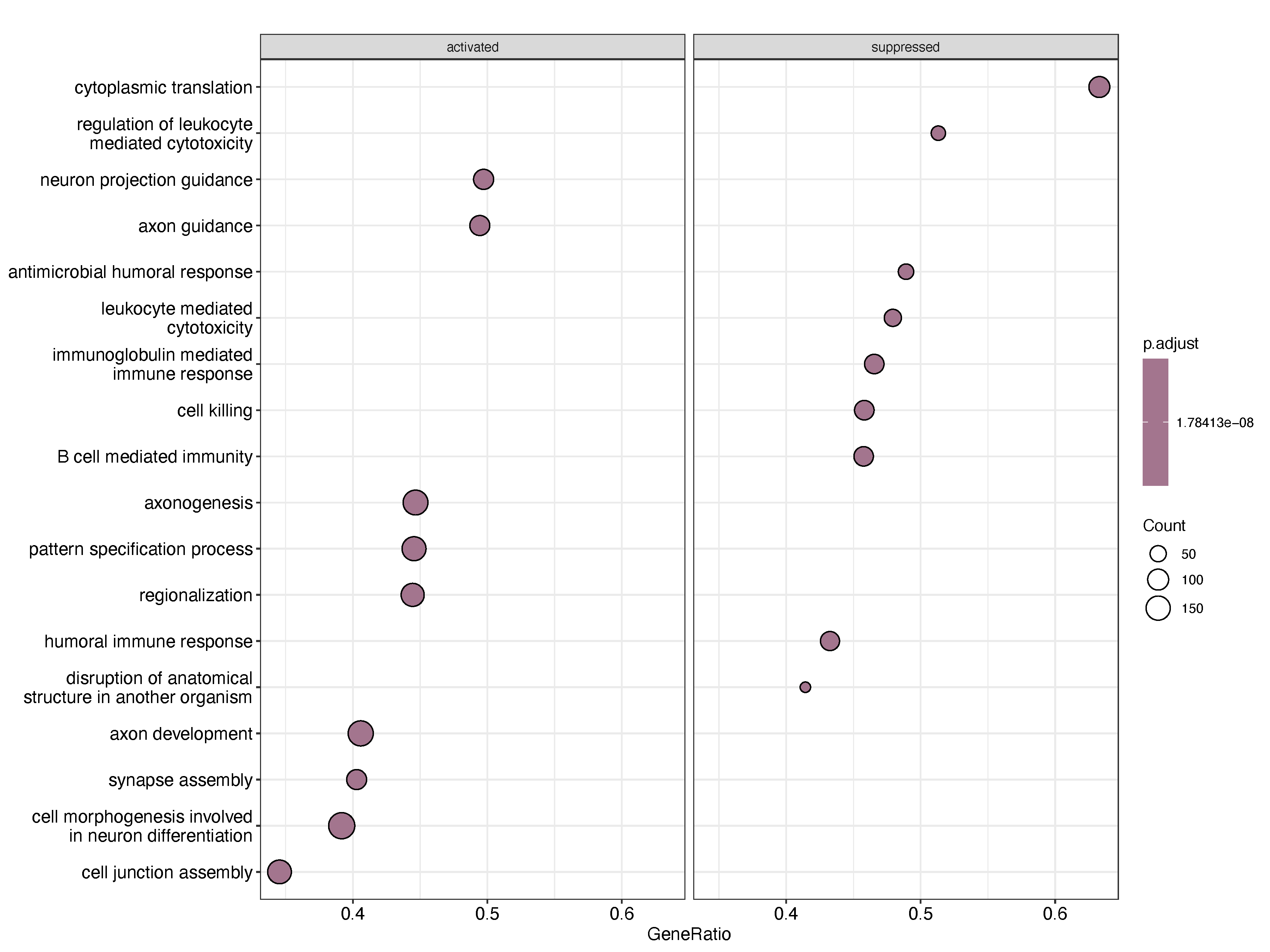
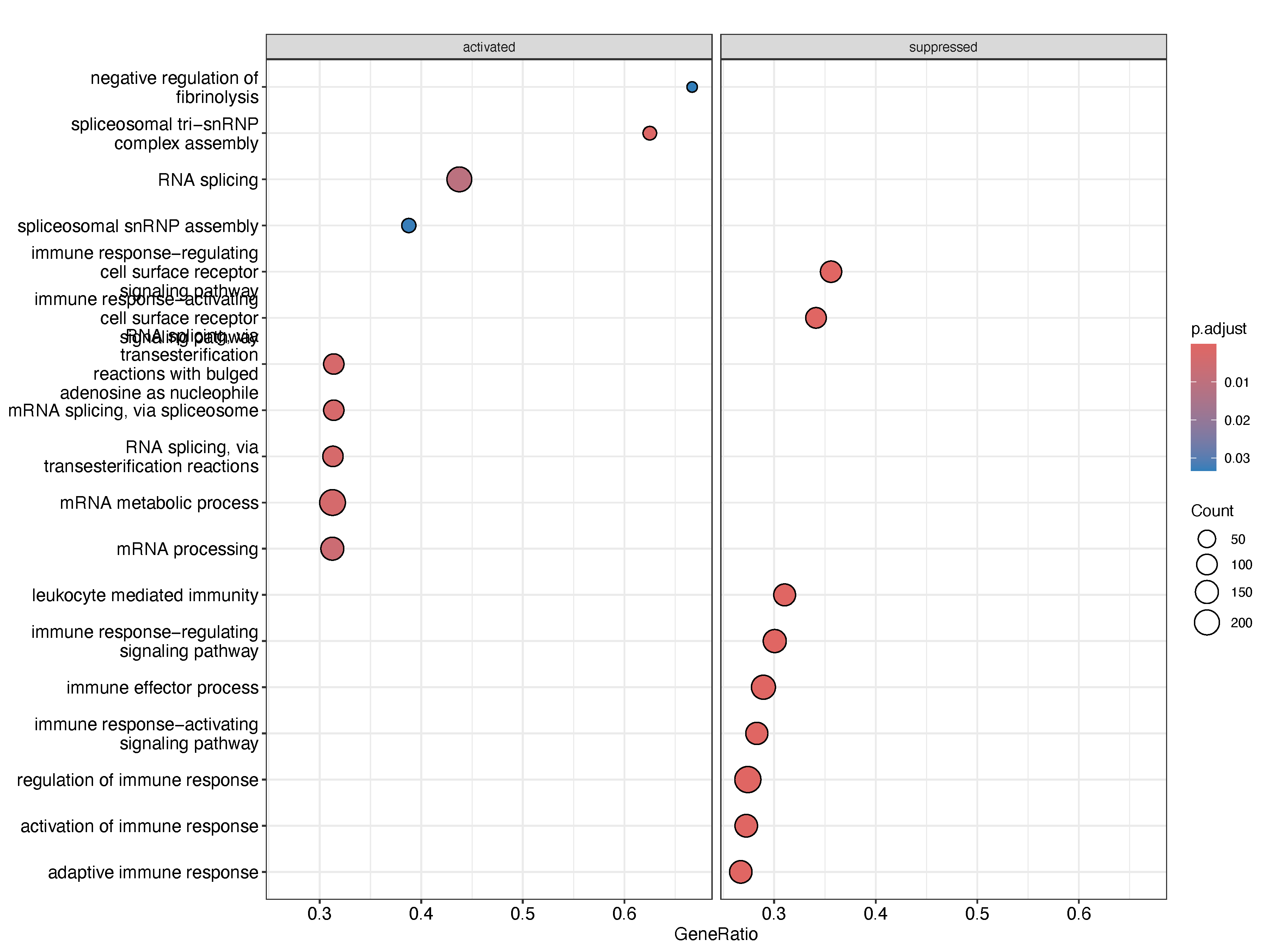
Paired analysis of relapse and baseline samples from the same individuals, conducted independently across two datasets, consistently revealed downregulation of immune-related functions upon relapse. Specifically, gene sets associated with B cell-mediated immunity, immunoglobulin-mediated immune response, and leukocyte-mediated immunity were significantly reduced in relapsed samples. This consistent suppression of humoral and cellular immune pathways may reflect several underlying biological mechanisms. One possibility is that clonal evolution during treatment and relapse selection favors immune-evasive subclones, which downregulate antigen presentation and antibody production to avoid immune surveillance. Alternatively, prolonged exposure to therapy may induce immunoediting or exhaustion of the immune microenvironment, leading to diminished support for anti-tumor immunity. These findings raise the possibility that immune dysfunction is not merely a consequence of relapse, but may represent a key contributor to disease progression and therapy resistance. Further functional studies will be necessary to determine whether reversing this immune suppression could improve post-relapse outcomes.
19.6 Box plots of top DEGs
pkgs <- c("ggthemes", "jhtools", "glue", "ggsci", "patchwork", "tidyverse",
          "circlize", "ComplexHeatmap", "SummarizedExperiment", "jhuanglabRNAseq",
          "viridis","ggrepel", "tidygraph","ggraph")
for (pkg in pkgs){
  suppressPackageStartupMessages(library(pkg, character.only = T))
}
project <- "leukemia"
dataset <- "meta"
species <- "human"
workdir <- glue("~/projects/{project}/analysis/{dataset}/{species}/figures/heatmap") |> checkdir()
setwd(workdir)
source("~/projects/leukemia/code/twist2_paper/used/0_load.R")

rdsobj <- read_rds("./paper_twist2_cdx2_g18/fig2/deg_volcano/deg_frame.rds")
group_twist2 <- rdsobj$frame_group_twist2
selectgenes <- rownames(group_twist2 |> slice_min(order_by = adj.P.Val, n = 6))

ans <- list()
for(i in selectgenes){
  genev <- assays(se)$tpm_remove_rnatype[i,] |> unlist()
  tmpdf <- tibble(
    sample_id = names(genev),
    value = genev
  ) |>
    left_join(colData(se)[,c("sample_id", "color_label")] |> as.data.frame()) |>
    mutate(color_label = factor(color_label, levels = totalcod))
  ans[[i]] <- ggplot(tmpdf, aes(x = color_label, y = value, fill = color_label)) +
    scale_fill_manual(values = metadata(se)$group_color$sample_label) +
    geom_boxplot() +
    ylab(i) +
    xlab("subtypes") +
    theme_few() +
    theme(axis.text.x = element_text(angle = 90, hjust = 1, vjust = 1))
}

pdf("~/projects/leukemia/analysis/meta/human/figures/heatmap/paper_twist2_cdx2_g18/fig2/degtop6.pdf",
    width = 12, height = 8)
  ans[[1]] + ans[[2]] + ans[[3]] + ans[[4]] + ans[[5]] + ans[[6]] +
  plot_layout(ncol = 3) +
  plot_annotation(title = "Top 6 DEGs in TWIST2-high group") &
  theme(legend.position = "none")
dev.off()