# Load required R packages silently
pkgs <- c("fs", "futile.logger", "configr", "ggpubr", "ggthemes",
          "jhtools", "glue", "ggsci", "patchwork", "tidyverse",
          "circlize", "ComplexHeatmap", "GenomicRanges", "jhuanglabRNAseq", "ggh4x")

for (pkg in pkgs) {
  suppressPackageStartupMessages(library(pkg, character.only = TRUE))
}10 clustering
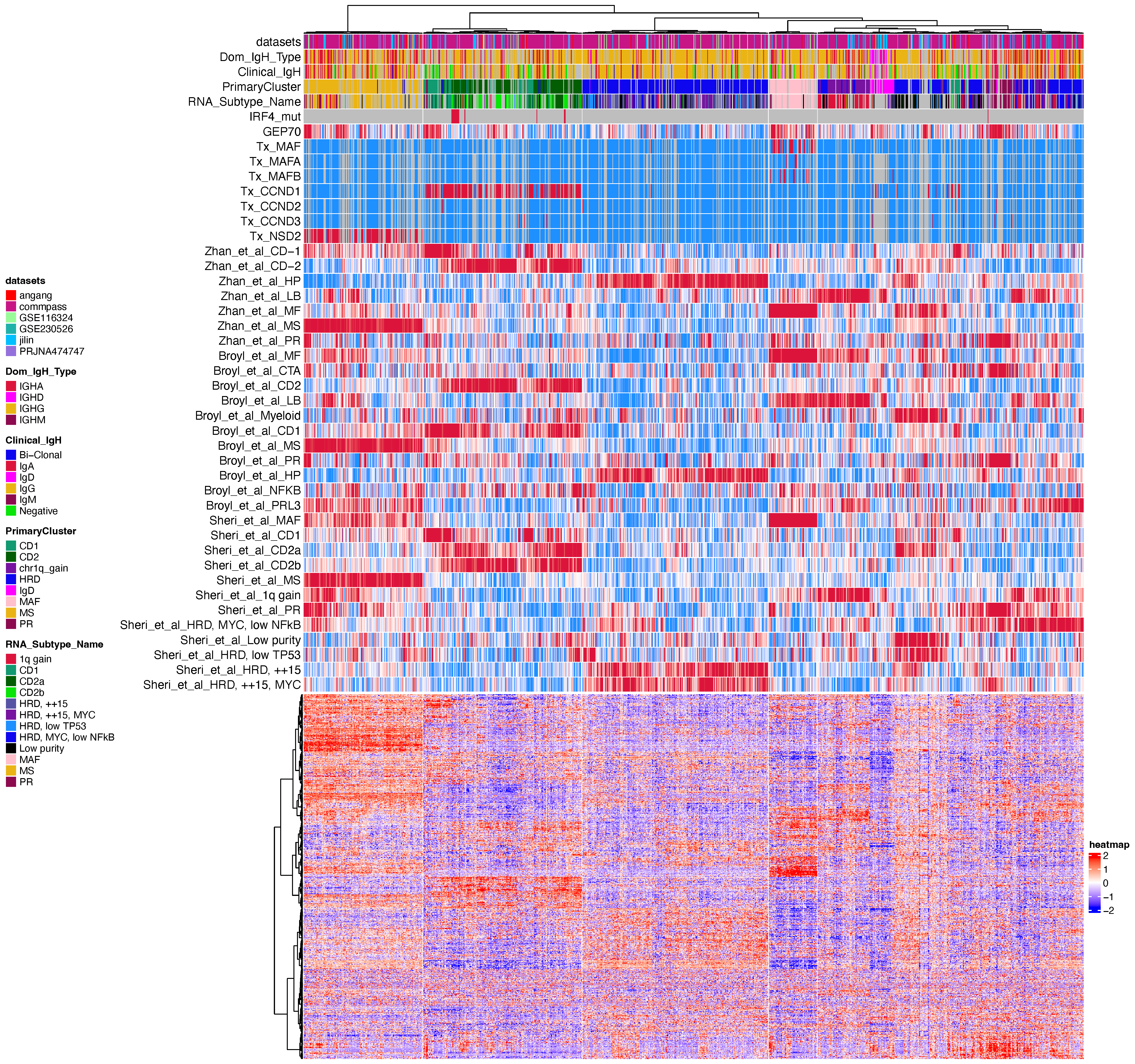
We performed unsupervised clustering and removed immunoglobulin genes in accordance with the methodology described in the CoMMpass study.
10.1 Overview
This document processes RNA-seq data for multiple myeloma (MM) to generate a heatmap visualization. The analysis includes loading required packages, setting up the working environment, preparing data, defining color schemes, and creating a complex heatmap with annotations.
10.2 Environment Setup
Set the project parameters, working directory, and random seed for reproducibility.
# Define project, dataset, and species
project <- "mm"
dataset <- "meta"
species <- "human"

# Create and set working directory
workdir <- glue("~/projects/{project}/analysis/{dataset}/{species}/rnaseq/figures/heatmap") |> checkdir()
setwd(workdir)

# Set random seed for reproducibility
set.seed(2025)
10.3 Data Loading
Load sample information and expression data from RDS files.
# Load sample information
df <- "~/projects/mm/docs/meta/sampleinfo/sampleinfo_jilin_commpass.rds" |> read_rds()

# Load heatmap-specific expression data
jinlin_commpass_heatmap_only <- "~/projects/mm/analysis/meta/human/rnaseq/exp/jinlin_commpass_heatmap_only.rds" |> read_rds()

# Load main expression data and convert to plotting format
dat_exp <- "~/projects/mm/analysis/meta/human/rnaseq/exp/mm_heatmap1117.rds" |>
  read_rds() |>
  convert_df_plot()

# Find common genes between datasets
cogene <- base::intersect(rownames(dat_exp), rownames(jinlin_commpass_heatmap_only))

# Filter sample metadata to match expression data columns
subdf <- df |> dplyr::filter(sample_id %in% colnames(dat_exp))
10.4 Color Configuration
Load color configurations from a YAML file and define custom color schemes for annotations.
# Load color configurations
config_fn <- "~/projects/mm/analysis/jilin/human/rnaseq/configs/colors.yaml"
config_list <- show_me_the_colors(config_fn, "all")

# Select specific color schemes
col <- config_list[c(
  "batch", "Clinical_IgH", "RNA_Subtype_Name",
  "PrimaryCluster", "Tx_MAF", "Tx_MAFA", "Tx_MAFB",
  "Tx_CCND1", "Tx_CCND2", "Tx_CCND3", "Tx_NSD2"
)]

# Define additional color mappings
col$Dom_IgH_Type <- col$Clinical_IgH
names(col$Dom_IgH_Type) <- c("IGHE", "IGHA", "IGHD", "IGHG", "IGHM", "others")
col$PrimaryCluster <- c(col$PrimaryCluster, "IgD" = "#FF00FF")
col$batch[] <- "gray"
col$datasets <- c(col$batch, "EGAD00001007813" = "gray", "HRA006164" = "red", bmc = "orange")
col$IRF4_mut <- c("TRUE" = "#DC143C", "FALSE" = "gray")

# Define color ramps for score annotations
all_scores <- c(
  "Zhan_et_al_CD-1", "Zhan_et_al_CD-2", "Zhan_et_al_HP", "Zhan_et_al_LB", "Zhan_et_al_MF",
  "Zhan_et_al_MS", "Zhan_et_al_PR", "Broyl_et_al_MF", "Broyl_et_al_CTA", "Broyl_et_al_CD2",
  "Broyl_et_al_LB", "Broyl_et_al_Myeloid", "Broyl_et_al_CD1", "Broyl_et_al_MS", "Broyl_et_al_PR",
  "Broyl_et_al_HP", "Broyl_et_al_NFKB", "Broyl_et_al_PRL3", "GEP70", "Sheri_et_al_MAF",
  "Sheri_et_al_CD1", "Sheri_et_al_CD2a", "Sheri_et_al_CD2b", "Sheri_et_al_MS",
  "Sheri_et_al_1q gain", "Sheri_et_al_PR", "Sheri_et_al_HRD, MYC, low NFkB",
  "Sheri_et_al_Low purity", "Sheri_et_al_HRD, low TP53", "Sheri_et_al_HRD, ++15",
  "Sheri_et_al_HRD, ++15, MYC"
)

for (i in all_scores) {
  col[[i]] <- circlize::colorRamp2(
    quantile(subdf[[i]], c(0.1, 0.5, 0.9), na.rm = TRUE),
    colors = c("#1E90FF", "white", "#DC143C")
  )
}
10.5 Heatmap Annotation
Prepare annotations for the heatmap based on selected metadata columns.
# Create output directory
out_dir <- "step1" |> checkdir()

# Define columns for annotation
all_col <- c("datasets",
             "Dom_IgH_Type", "Clinical_IgH", "PrimaryCluster", "RNA_Subtype_Name",
             "IRF4_mut", "GEP70",
             "Tx_MAF", "Tx_MAFA", "Tx_MAFB", "Tx_CCND1", "Tx_CCND2", "Tx_CCND3", "Tx_NSD2",
             all_scores)

# Create heatmap annotation object
hasub2 <- HeatmapAnnotation(
  df = subdf[, all_col] |> as.data.frame(),
  annotation_name_side = "left",
  show_legend = all_col %in% c("datasets", "Dom_IgH_Type",
                               "Clinical_IgH", "PrimaryCluster",
                               "RNA_Subtype_Name"),
  col = col
)
10.6 Heatmap Generation
Generate and save a complex heatmap with custom annotations.
# Prepare metadata for heatmap
hdf <- subdf[, c("sample_id", "cn_name", "PrimaryCluster", "RNA_Subtype_Name",
                 "tumor_descriptor", "Tx_CCND1", "Tx_CCND2", "Tx_CCND3")] |>
  mutate(
    CCNDx = Tx_CCND1 | Tx_CCND2 | Tx_CCND3,
    cn_name = case_when(
      is.na(cn_name) ~ str_extract(sample_id, pattern = "MMRF_\\d+|MM\\d+"),
      TRUE ~ cn_name
    )
  ) |>
  dplyr::select(-c(Tx_CCND1, Tx_CCND2, Tx_CCND3))

# Generate heatmap
quick_heatmap(
  dat_exp[cogene, subdf$sample_id],
  hasub2,
  outdir = out_dir,
  hdf = hdf,
  top_var_percent = 0.9,
  keep_annotation = TRUE,
  column_split = 16,
  height = 15,
  out_put_rds = TRUE,
  cluster_columns = TRUE,
  show_column_names = FALSE
)
10.7 two-step clustering
Why did we adopt a two-step clustering approach? We observed that the gene expression patterns of the MAF and NSD2 groups were particularly distinct. When all samples were clustered together using the most highly variable genes, the majority of these genes were associated with the MAF and NSD2 groups. As a result, the clustering was dominated by these two groups, potentially masking the variability and distinct features of other subgroups.
A similar issue arose during differential expression analysis. When comparing one group against all others, the differentially expressed genes were consistently enriched for those distinguishing the MAF and NSD2 groups, again overshadowing differences among the remaining groups.
To address this, we first separated the MAF and NSD2 groups from the dataset and then performed clustering on the remaining samples. This strategy allowed us to identify highly variable genes that better capture the characteristics of the other subgroups, leading to a more balanced and informative clustering outcome.
10.8 Unsupervised cluster
10.9 Consensus clustering heatmap
Following the initial clustering step, we removed clusters exhibiting dominant or well-characterized features in order to reduce confounding influences and better highlight the heterogeneity among the remaining samples. The results of the second round of clustering are shown below:
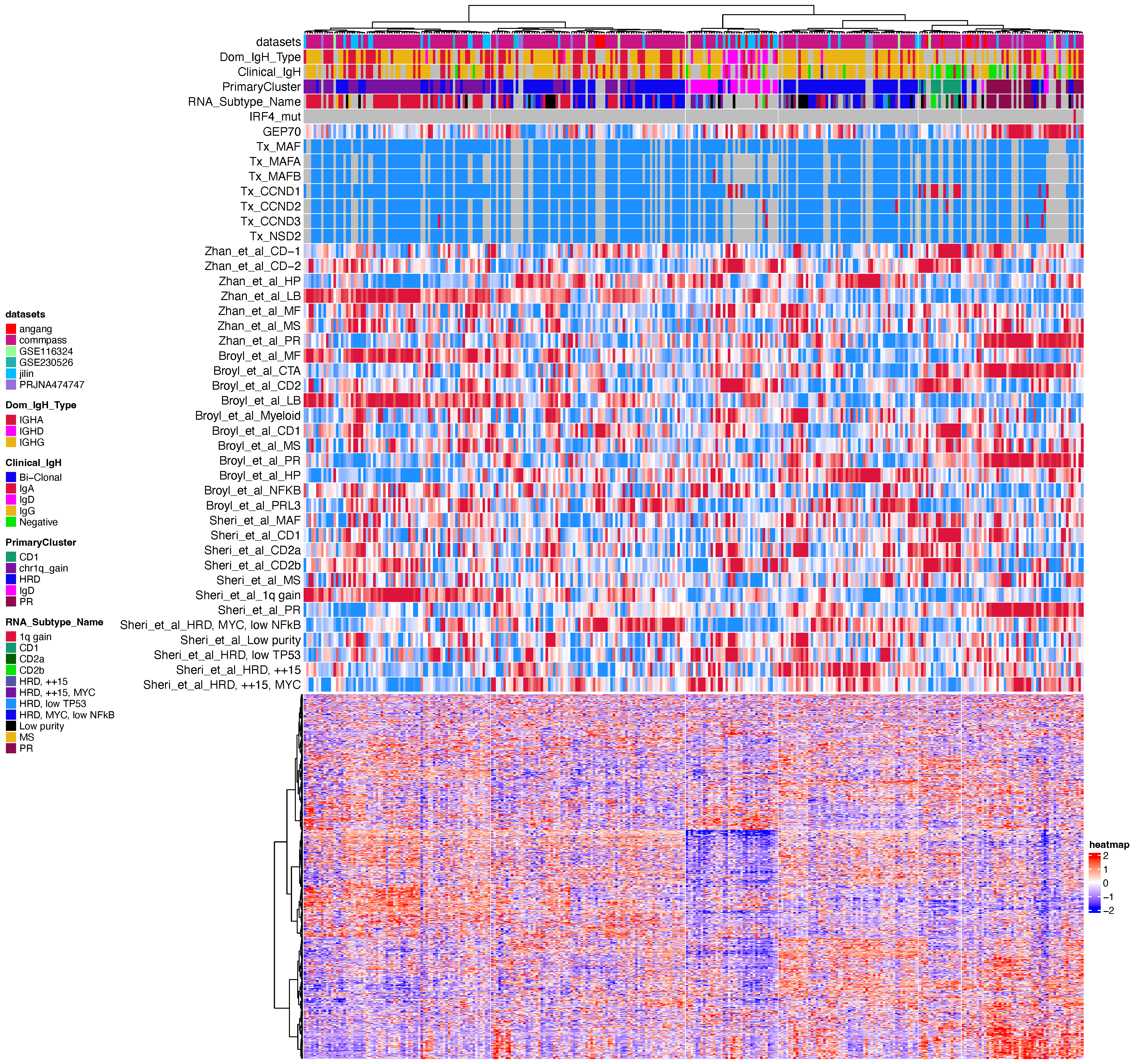
Based on the combined results from the two-stage clustering, we annotated a total of 12 distinct groups. To evaluate the biological coherence and consistency of these subtypes, we scored each group using gene sets derived from two previously published studies, assessing their alignment with established molecular annotations.