12 Dimensionality Reduction

Dimensionality reduction is a technique used to reduce the number of random variables (features or dimensions) in a dataset, while retaining as much important information as possible.

It transforms high-dimensional data into a lower-dimensional space (often 2D or 3D), making it easier to: Visualize Analyze Model

This is especially useful when working with complex datasets like gene expression data, images, text, or any data with many features.

High-dimensional data can cause several issues:

Curse of dimensionality : More features mean more computational cost and risk of overfitting.
Redundant or correlated features : Many features might provide similar information.
Hard to visualize : Humans can’t easily interpret data with hundreds or thousands of dimensions.

pkgs <- c("fs", "futile.logger", "configr", "ggpubr", "ggthemes",
          "jhtools", "glue", "ggsci", "patchwork", "tidyverse",
          "circlize", "ComplexHeatmap", "GenomicRanges", "jhuanglabRNAseq", "ggh4x")
for (pkg in pkgs){
  suppressPackageStartupMessages(library(pkg, character.only = T))
}
project <- "mm"
dataset <- "meta"
species <- "human"
workdir <- glue("~/projects/{project}/analysis/{dataset}/{species}/rnaseq/figures/heatmap") |> checkdir()
setwd(workdir)
set.seed(2025)
# loading data
sfn <- "~/projects/mm/docs/meta/sampleinfo/sampleinfo_jilin_commpass.rds"
sampleinfo_raw <- read_rds(sfn)
dat_raw <- "~/projects/mm/analysis/meta/human/rnaseq/exp/mm_heatmap1117.rds" |>
  read_rds() |> convert_df_plot()
heatmap_genes <- "~/projects/mm/analysis/meta/human/rnaseq/figures/heatmap/step1/sampleinfo_0.9.xlsx" |>
  readxl::read_xlsx(sheet = "heatmapeGenes")
dat_exp <- dat_raw[heatmap_genes$gene_name, ] |> t()

sampleinfo <- sampleinfo_raw %>%
  filter(sample_id %in% rownames(dat_exp)) %>%
  arrange(match(sample_id, rownames(dat_exp))) %>%
  select(sample_id, subtypes)

col_subt <- c("Low_purity" = "black", "MS" = "#ebb415",
              "CD1a1" = "#129a71", "CD1a2" = "#8ff7c1", "CD1b" = "#09e409", "CD2" = "#035e03",
              "PR" = "#8d0a4f", "IgD" = "#FF00FF", "chr1qgain" = "#DC143C", "HRD_chr1qgain" = "#5653a5",
              "HRD_MYC_lowNFkB" = "#7713a0", "HRD_lowTP53" = "#1E90FF", "HRD15" = "#6fade8",
              "MAF" = "#bf457e")
sampleinfo$color_subtypes <- col_subt[sampleinfo$subtypes]
#
pca_raw <- prcomp(dat_exp, scale. = TRUE)
pca_mat <- as.data.frame(pca_raw$x[, 1:2])
tsne_raw <- Rtsne::Rtsne(dat_exp, perplexity = 30, max_iter = 1000,
                     verbose = FALSE, check_duplicates = FALSE)
tsne_mat <- as.data.frame(tsne_raw$Y)
colnames(tsne_mat) <- c("tSNE_1", "tSNE_2")
rownames(tsne_mat) <- rownames(dat_exp)
umap_raw <- umap::umap(dat_exp, n_neighbors = 15,
                    n_components = 2, min_dist = 0.1,
                    metric = "euclidean")
umap_mat <- as.data.frame(umap_raw$layout)
colnames(umap_mat) <- c("UMAP_1", "UMAP_2")
rownames(umap_mat) <- rownames(dat_exp)
#PCA
pdf("pca_subtypes.pdf", width = 6, height = 6)
  plot(pca_mat, pch = 16, cex = 0.6,
     xlab = "Principal Component 1",
     ylab = "Principal Component 2",
     col = sampleinfo$color_subtypes,
     main = "Principal Component Analysis")
  legend("topright", legend = unique(sampleinfo$subtypes),
       col = unique(sampleinfo$color_subtypes), pch = 16, cex = 0.6)
dev.off()

pdf("tsne_subtypes.pdf", width = 6, height = 4)
  ggplot(tsne_mat, aes(x = tSNE_1, y = tSNE_2, color = sampleinfo$subtypes)) +
    geom_point(size = 0.8) +
    theme_classic() +
    scale_color_manual(values = col_subt) +
    guides(color = guide_legend(override.aes = list(size = 3)))
dev.off()

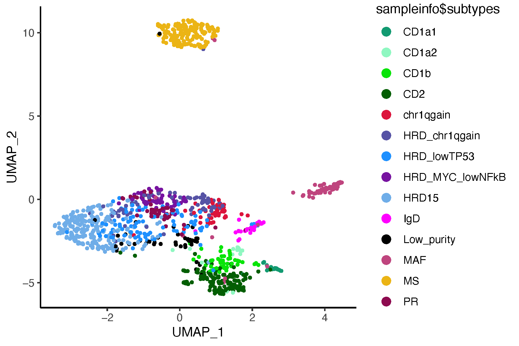
pdf("umap_subtypes.pdf", width = 6, height = 4)
  ggplot(umap_mat, aes(x = UMAP_1, y = UMAP_2, color = sampleinfo$subtypes)) +
    geom_point(size = 0.8) +
    theme_classic() +
    scale_color_manual(values = col_subt) +
    guides(color = guide_legend(override.aes = list(size = 3)))
dev.off()

12.1 PCA figure

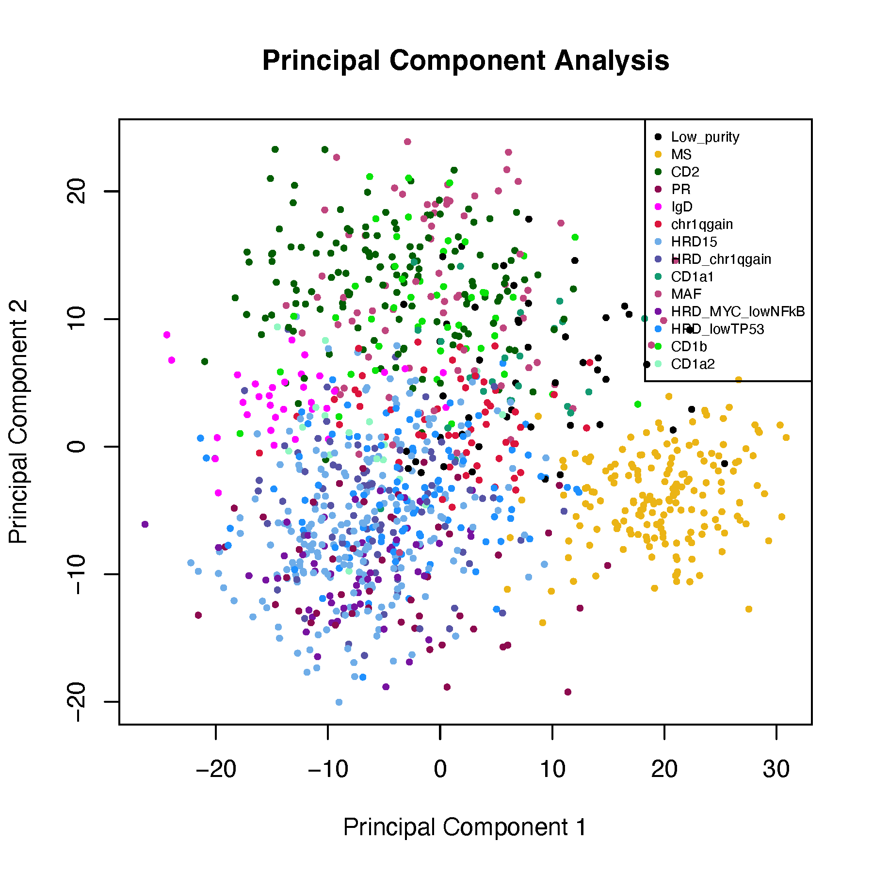
12.2 tSNE figure

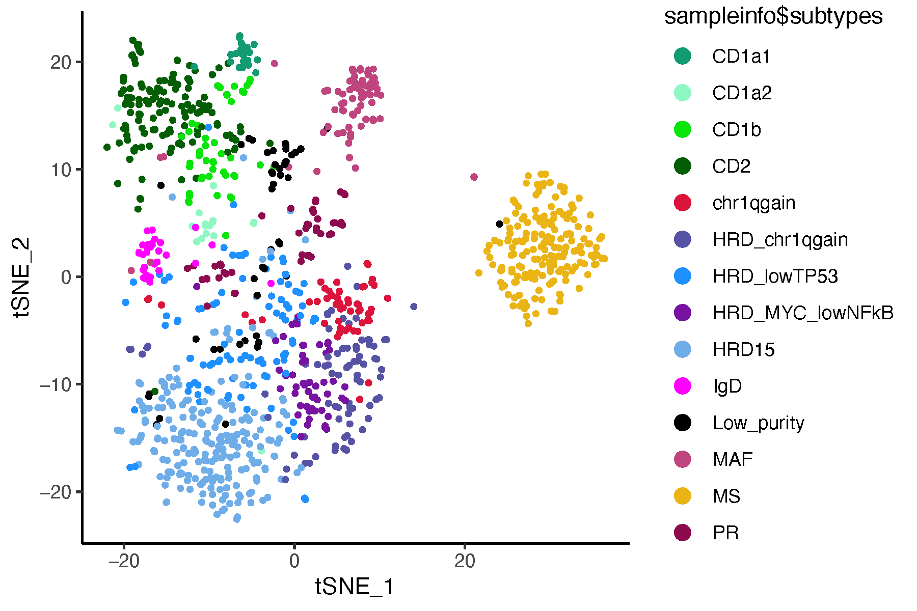
12.3 UMAP figure