pkgs <- c("fs", "futile.logger", "configr", "stringr", "ggpubr", "ggthemes",
          "jhtools", "glue", "ggsci", "patchwork", "tidyverse", "gplots")
for (pkg in pkgs){
  suppressPackageStartupMessages(library(pkg, character.only = T))
}

merged_sinfo <- read_rds("~/projects/mm/docs/meta/sampleinfo/sampleinfo_jilin_commpass.rds")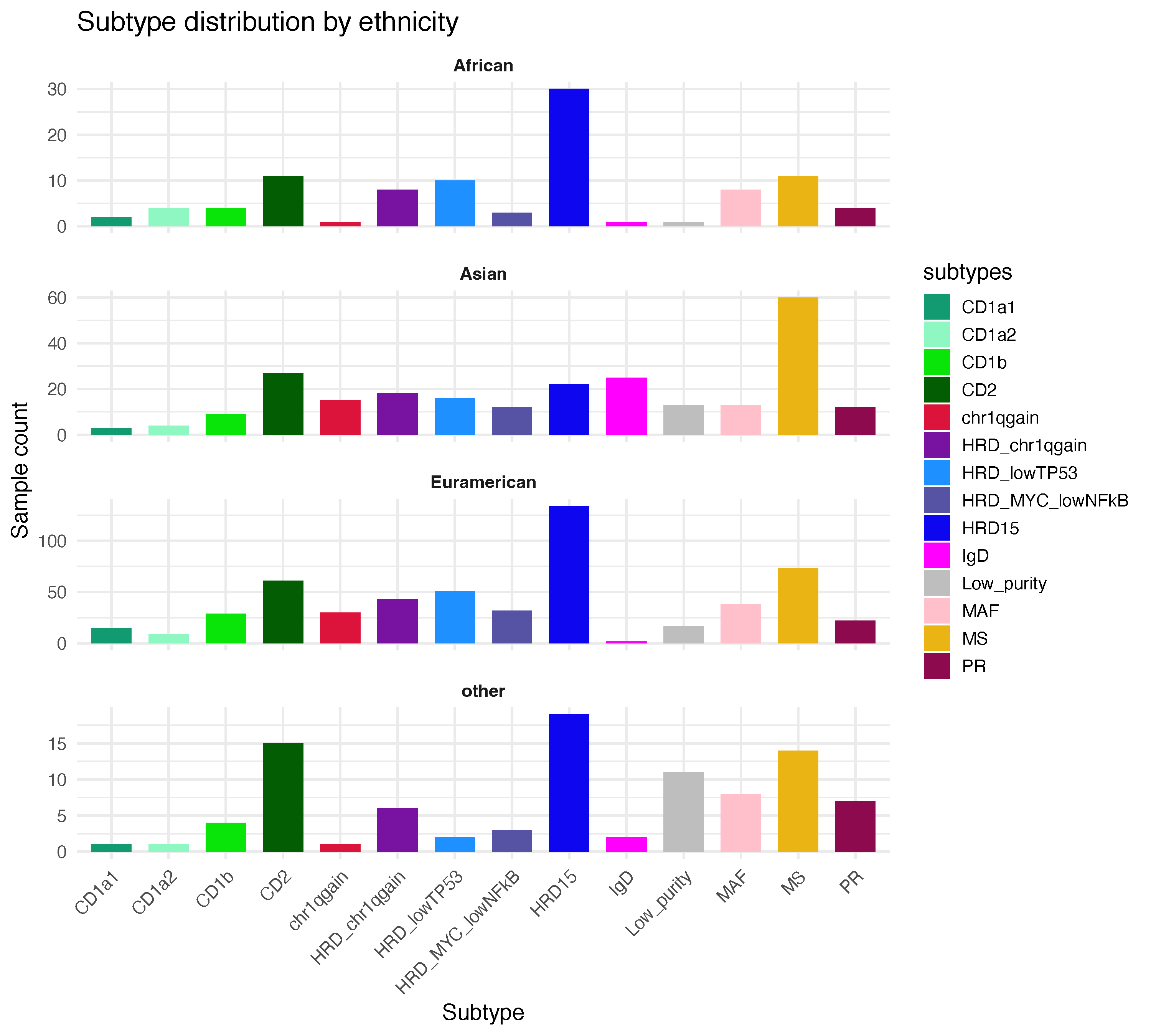
plot_data <- merged_sinfo %>% dplyr::count(ethnicity, subtypes) %>% na.omit() 24 Ethnicity groups in this study
Population-related differences represent a key but underexplored dimension in the study of multiple myeloma (MM). Epidemiological data have shown that the incidence of MM among Asian populations is approximately half that observed in Western populations, while individuals of African descent exhibit a two-fold higher incidence. These striking disparities suggest that ancestry-associated genetic and/or environmental factors may influence MM pathogenesis. Moreover, molecular subtypes of MM appear to vary in distribution across populations, further highlighting the potential relevance of population background. Notably, the CoMMpass dataset (currently the largest publicly available resource for MM) includes only ~3% of patients of Asian ancestry, posing a significant limitation for population-level comparisons. In this chapter, we investigate the molecular subtype landscape of MM across different ancestral groups, incorporating a newly curated cohort of Asian patients. Our analysis aims to advance the current understanding of population-specific features and their biological implications in MM.
24.1 Subtype differences
We first summarized the molecular subtypes identified in this study, the procedures are as follows:
Get data for plot:
Show the data as barplot:
# set colors
# config_fn = "~/projects/mm/analysis/jilin/human/rnaseq/configs/colors.yaml"
# all_color <- show_me_the_colors(config_fn, "RNA_Subtype_Name")
# names(all_color) <- c("CD1", "CD2", "CD_no_IgH", "Low_purity", "HRD", "HRD_1q_gain",
#                       "HRD_chr11", "IgD", "MS", "PR", "MAF", "1q_gain")
# all_color["IgD"] <- "#FF00FF"
all_color <- c("Low_purity" = "grey", "MS" = "#ebb415", "MAF" = "pink", "PR" = "#8d0a4f",
               "CD1a1" = "#129a71", "CD1a2" = "#8ff7c1", "CD1b" = "#09e409", "CD2" = "#035e03",
               "IgD" = "#FF00FF", "chr1qgain" = "#DC143C", "HRD_MYC_lowNFkB" = "#5653a5",
               "HRD_chr1qgain" = "#7713a0", "HRD_lowTP53" = "#1E90FF", "HRD15" = "#0e06ee")

setwd("/cluster/home/yjliu_jh/projects/mm/output/eth_diff")
testg <- ggplot(plot_data, aes(x = subtypes, y = n, fill = subtypes)) +
  geom_bar(stat = "identity", width = 0.7) +
  facet_wrap(~ ethnicity, ncol = 1, scales = "free_y") +
  scale_fill_manual(values = all_color) +
  theme_minimal(base_size = 14) +
  theme(
    strip.text = element_text(face = "bold"),
    axis.text.x = element_text(angle = 45, hjust = 1),
    panel.spacing = unit(1, "lines")
  ) +
  labs(x = "Subtype", y = "Sample count", title = "Subtype distribution by ethnicity")
ggsave("subtype_counts.pdf", testg, width = 10, height = 9)
The figure below summarizes the distribution of molecular subtypes across different population groups in terms of sample count.
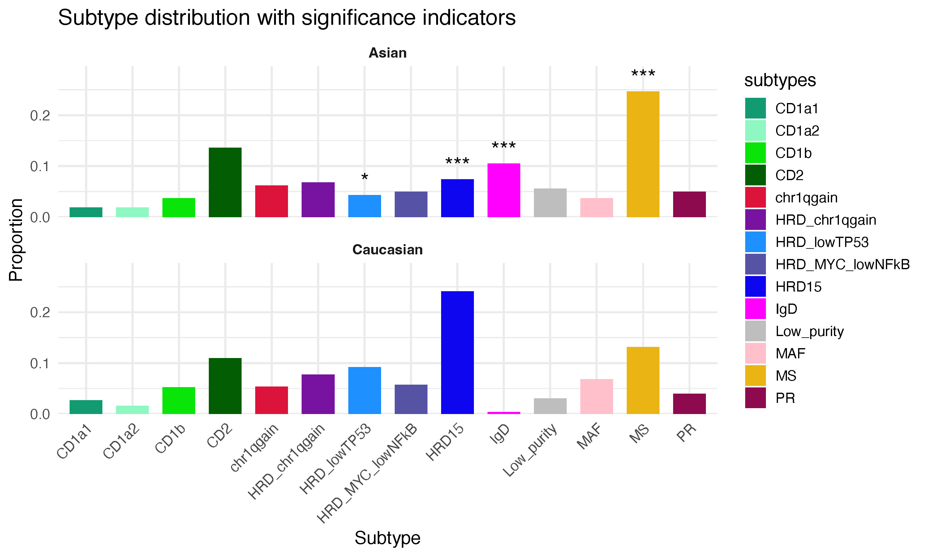
Next, we compared the Asian population (including the newly profiled Asian cohort) from this study with Western cohorts which constitute the majority of existing MM studies. Aiming to identify features that may be unique or enriched in Asian patients, particularly with respect to subtype prevalence and distribution, we have performed subtype-wise differential test as follows:
Fisher tests were used to estimate a p value according to the data proportions:
merged_sinfo2 <- merged_sinfo[merged_sinfo$ethnicity %in% c("Asian", "Caucasian"), c("subtypes", "ethnicity", "batch")] %>% na.omit()
plot_data2 <- merged_sinfo2 %>% dplyr::count(ethnicity, subtypes) %>% group_by(ethnicity) %>%
  mutate(freq = n / sum(n)) %>% ungroup()
subtypes <- unique(merged_sinfo2$subtypes)
pvals <- lapply(subtypes, function(st) {
  tab <- merged_sinfo2 %>%
    mutate(is_target = ifelse(subtypes == st, "Target", "Other")) %>%
    dplyr::count(ethnicity, is_target) %>%
    pivot_wider(names_from = is_target, values_from = n, values_fill = 0) %>%
    column_to_rownames("ethnicity") %>%
    as.matrix()
  pval <- fisher.test(tab)$p.value
  data.frame(subtypes = st, p = pval)
}) %>%
  bind_rows() %>%
  mutate(star = case_when(
    p < 0.001 ~ "***",
    p < 0.01 ~ "**",
    p < 0.05 ~ "*",
    TRUE ~ ""
  ))
Subtypes with significant proportion change are marked by asterisks:
plot_data2 <- left_join(plot_data2, pvals, by = "subtypes")
plot_data2$star[plot_data2$ethnicity != "Asian"] <- ""

# plot
testg2 <- ggplot(plot_data2, aes(x = subtypes, y = freq, fill = subtypes)) +
  geom_bar(stat = "identity", width = 0.7) +
  scale_y_continuous(expand = expansion(mult = c(0, 0.2))) +
  facet_wrap(~ ethnicity, ncol = 1) +
  geom_text(aes(label = star), vjust = -0.4, size = 6) +
  scale_fill_manual(values = all_color) +
  theme_minimal(base_size = 14) +
  theme(
    strip.text = element_text(face = "bold"),
    axis.text.x = element_text(angle = 45, hjust = 1),
    panel.spacing = unit(1, "lines")
  ) +
  labs(x = "Subtype", y = "Proportion", title = "Subtype distribution with significance indicators")

ggsave("subtype_counts_freq_sig.pdf", testg2, width = 10, height = 6)
This figure presents the relative proportions of each subtype by population, along with the subtypes exhibiting statistically significant differences.
24.1.1 Functional differences across the subtypes
Changes in subtype frequency may reflect differences in genetic background, environmental exposures, or their interactions. Alternatively, the same subtype may exhibit distinct transcriptomic or molecular features across populations, indicating further stratification within known subgroups. Investigating such population-specific variation may enhance our understanding of ancestry-related disease biology. To this end, we performed comparative analyses focusing on the subtypes that showed significant differences in frequency between Asian and Western patients. Among the 12 defined subtypes, three (classical HRD, MS and the IgD-enriched groups) showed pronounced differences in relative frequency across populations. For each of these subtypes, we further analyzed transcriptomic differences between Asian and Western patients.
There are multiple methodological choices and parameter settings available for differential expression analysis, each of which may introduce slight variations in the results. To ensure clarity and reproducibility, we outline our analysis procedure in detail below:
To reduce confounding and ensure consistent gene-level annotations, we restricted our analysis to genes with official gene symbols, and filtered out genes with low expression across samples.
pkgs <- c("fs", "futile.logger", "configr", "stringr", "ggpubr", "ggthemes",
          "jhtools", "glue", "ggsci", "patchwork", "tidyverse", "dplyr",
          "SummarizedExperiment", "jhuanglabRNAseq", "DESeq2", "gplots",
          "matrixStats", "Matrix", "dendextend", "ComplexHeatmap", "rstatix",
          "clusterProfiler", "DOSE", "org.Hs.eg.db", "EnhancedVolcano",
          "GseaVis")
for (pkg in pkgs){
  suppressPackageStartupMessages(library(pkg, character.only = T))
}


# set workdir
setwd("/cluster/home/yjliu_jh/projects/mm/output/eth_diff")
merged_sinfo <- read_rds("~/projects/mm/docs/meta/sampleinfo/sampleinfo_jilin_commpass.rds")

# update gene name annotation
hugo_anno <- readr::read_delim("/cluster/home/yjliu_jh/projects/mm/data/hgnc_complete_set.txt",
                               col_types = cols(intermediate_filament_db = col_character()))
hugo_anno <- hugo_anno[, c("symbol", "ensembl_gene_id", "locus_group")] %>% as.data.frame()
colnames(hugo_anno)[2] <- "gene_id"

# load counts
mmdatasets <- c("jilin", "commpass", "public", "HRA005897")
count_files <- glue::glue("/cluster/home/jhuang/projects/mm/analysis/{mmdatasets}/human/rnaseq/exp/tables/{mmdatasets}_human_counts.csv")
total_counts_list <- lapply(count_files[file.exists(count_files)], read_csv)
names <- mmdatasets[file.exists(count_files)]
counts_all <- total_counts_list[[1]]
for (i in 2:length(total_counts_list)) {
  counts_all <- bind_cols(counts_all, total_counts_list[[i]][, -(1:2)])
}

# load new gene symbol info
hugo_anno <- readr::read_delim("/cluster/home/yjliu_jh/projects/mm/data/hgnc_complete_set.txt",
                               col_types = cols(intermediate_filament_db = col_character()))
symbol_anno <- hugo_anno |> separate_rows(prev_symbol, sep = "\\|") |> as.data.frame()
hugo_anno <- hugo_anno[, c("symbol", "ensembl_gene_id", "locus_group")] %>% as.data.frame()
colnames(hugo_anno)[2] <- "gene_id"

# prepare counts data
counts_all <- counts_all[, -2] %>% left_join(hugo_anno) %>% na.omit() %>%
  dplyr::select(-c(gene_id, locus_group)) %>% as.data.frame() %>% remove_rownames() %>%
  column_to_rownames(var = "symbol") %>% as.matrix() %>% round()
counts_primary2 <- counts_all[, colnames(counts_all) %in% merged_sinfo$sample_id[!is.na(merged_sinfo$subtypes)]]
sinfo_primary2 <- merged_sinfo[, c("sample_id", "datasets", "batch", "ethnicity", "subtypes")] %>% unique() %>% as.data.frame()
rownames(sinfo_primary2) <- sinfo_primary2$sample_id
sinfo_primary2 <- sinfo_primary2[colnames(counts_primary2), ]
sinfo_comp <- sinfo_primary2[sinfo_primary2$ethnicity %in% c("Asian", "Caucasian"), ]
rna_lib_large <- read_rds("/cluster/home/yjliu_jh/projects/mm/output/rna_lib_mm_samples.rds")
sinfo_comp <- left_join(sinfo_comp, rna_lib_large)
rownames(sinfo_comp) <- sinfo_comp$sample_id
Since population group and dataset origin were highly correlated in this study, we avoided applying full batch correction to prevent the suppression of genuine population-driven differences. Instead, we corrected only for library preparation type (mRNA vs. total RNA) as a technical covariate.
# construct dds object - HRD chr15++
sinfo_hrd <- sinfo_comp[sinfo_comp$subtypes %in% "HRD15", ]
counts_hrd <- counts_primary2[, rownames(sinfo_hrd)]
dds_hrd <- DESeqDataSetFromMatrix(counts_hrd, sinfo_hrd, ~ rna_type + ethnicity)
keep <- rowSums(counts(dds_hrd) >= 5) > ceiling(0.2 * ncol(dds_hrd))
dds_hrd <- dds_hrd[keep, ]
keep2 <- rowSums(counts(dds_hrd) == 0) < ceiling(0.5 * ncol(dds_hrd))
dds_hrd <- dds_hrd[keep2, ]
dds_hrd <- DESeq(dds_hrd)

# construct dds object - IgD
sinfo_igd <- sinfo_comp[sinfo_comp$subtypes %in% "IgD", ]
counts_igd <- counts_primary2[, rownames(sinfo_igd)]
dds_igd <- DESeqDataSetFromMatrix(counts_igd, sinfo_igd, ~ rna_type + ethnicity)
keep <- rowSums(counts(dds_igd) >= 5) > ceiling(0.2 * ncol(dds_igd))
dds_igd <- dds_igd[keep, ]
keep2 <- rowSums(counts(dds_igd) == 0) < ceiling(0.5 * ncol(dds_igd))
dds_igd <- dds_igd[keep2, ]
dds_igd <- DESeq(dds_igd)

# construct dds object - MS
sinfo_ms <- sinfo_comp[sinfo_comp$subtypes %in% "MS", ]
counts_ms <- counts_primary2[, rownames(sinfo_ms)]
dds_ms <- DESeqDataSetFromMatrix(counts_ms, sinfo_ms, ~ rna_type + ethnicity)
keep <- rowSums(counts(dds_ms) >= 5) > ceiling(0.2 * ncol(dds_ms))
dds_ms <- dds_ms[keep, ]
keep2 <- rowSums(counts(dds_ms) == 0) < ceiling(0.5 * ncol(dds_ms))
dds_ms <- dds_ms[keep2, ]
dds_ms <- DESeq(dds_ms)

# construct dds object - HRD chr15++
sinfo_hrd2 <- sinfo_comp[sinfo_comp$subtypes %in% "HRD_lowTP53", ]
counts_hrd2 <- counts_primary2[, rownames(sinfo_hrd2)]
dds_hrd2 <- DESeqDataSetFromMatrix(counts_hrd2, sinfo_hrd2, ~ rna_type + ethnicity)
keep <- rowSums(counts(dds_hrd2) >= 5) > ceiling(0.2 * ncol(dds_hrd2))
dds_hrd2 <- dds_hrd2[keep, ]
keep2 <- rowSums(counts(dds_hrd2) == 0) < ceiling(0.5 * ncol(dds_hrd2))
dds_hrd2 <- dds_hrd2[keep2, ]
dds_hrd2 <- DESeq(dds_hrd2)
# order and add columns to the results
add_col <- function(data){
data$gene_name <- rownames(data)
data$absFC <- abs(data$log2FoldChange)
data <- data[order(data$pvalue), ]
data2 <- left_join(as.data.frame(data), hugo_anno[, c("symbol", "gene_id")], by = c("gene_name" = "symbol"))
data$ensembl_id <- data2$gene_id
data
}
# get result for subtype-wise comparison
res_hrd <- add_col(results(dds_hrd, c("ethnicity", "Asian", "Caucasian")))
GSEA2 <- res_hrd$log2FoldChange
names(GSEA2) <- as.character(rownames(res_hrd))
GSEA2 <- sort(GSEA2, decreasing = TRUE)
res_igd <- add_col(results(dds_igd, c("ethnicity", "Asian", "Caucasian")))
GSEA3 <- res_igd$log2FoldChange
names(GSEA3) <- as.character(rownames(res_igd))
GSEA3 <- sort(GSEA3, decreasing = TRUE)
res_ms <- add_col(results(dds_ms, c("ethnicity", "Asian", "Caucasian")))
GSEA4 <- res_ms$log2FoldChange
names(GSEA4) <- as.character(rownames(res_ms))
GSEA4 <- sort(GSEA4, decreasing = TRUE)
res_hrd2 <- add_col(results(dds_hrd2, c("ethnicity", "Asian", "Caucasian")))
GSEA5 <- res_hrd2$log2FoldChange
names(GSEA5) <- as.character(rownames(res_hrd2))
GSEA5 <- sort(GSEA5, decreasing = TRUE)
# comp input
ccres <- compareCluster(geneCluster = list(HRD_15amp = GSEA2, IgD = GSEA3, MS = GSEA4, HRD_lowTP53 = GSEA5),
fun = gseGO, OrgDb = org.Hs.eg.db, keyType = "SYMBOL", ont = "BP",
minGSSize = 5, maxGSSize = 1000, pvalueCutoff = 0.1)
pdf("four_comp.pdf", width = 10, height = 10)
dotplot(ccres)
dev.off()We focused on the three subtypes with the most significant population-level differences, as shown in the figure above. For each subtype, we conducted gene-level differential expression analysis between Asian and Western patients, and used the compareCluster() function to visualize enriched biological pathways. The top five significantly enriched Gene Ontology (GO) terms for each subtype are shown as representative results.
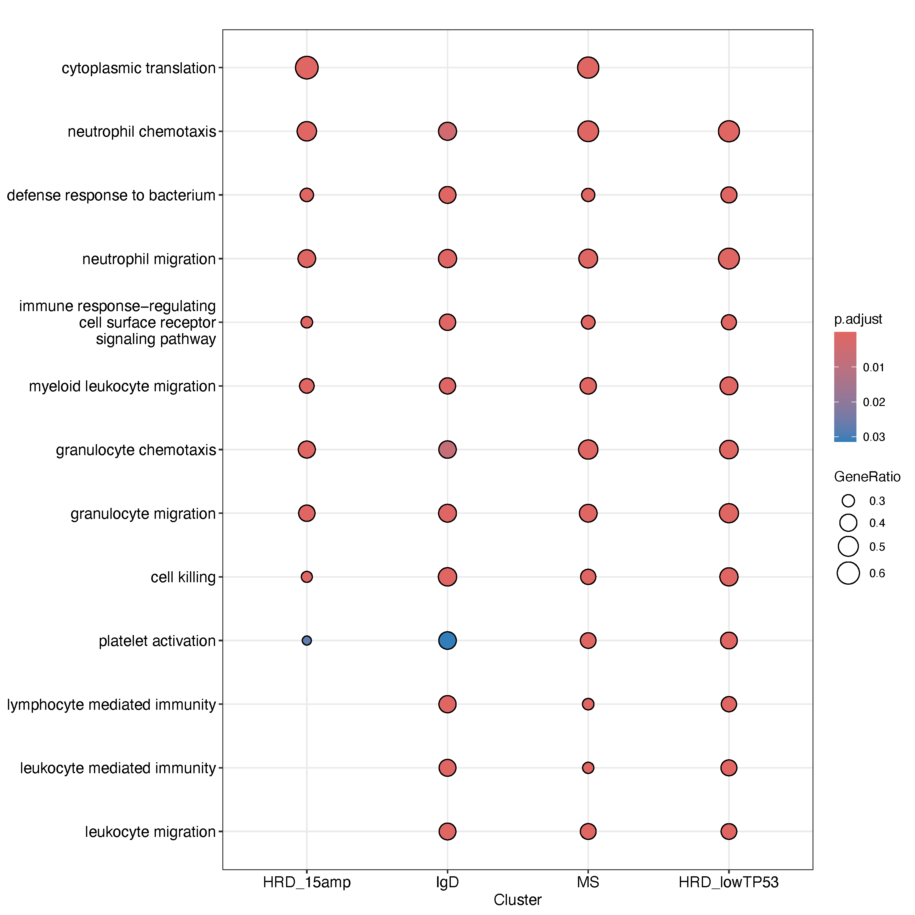
Gene set enrichment analysis revealed that Asian patients with HRD-type multiple myeloma exhibited broad upregulation of immune- and inflammation-related functions compared to White patients within the same subtype. Enriched pathways included lymphocyte-mediated immunity, platelet activation, granulocyte and neutrophil chemotaxis, cytoplasmic translation, neutrophil migration, and cell killing. This pattern suggests that the tumor microenvironment in Asian HRD samples may be more immunologically active or inflamed.
The increased expression of genes associated with B and T cell-mediated immunity and cytotoxic effector functions points toward a heightened immune surveillance or inflammatory state. Upregulation of granulocyte and neutrophil chemotaxis implies enhanced innate immune cell recruitment, while platelet activation may reflect interplay between coagulation and immune activation—a known feature in some hematologic malignancies. The enrichment of cytoplasmic translation pathways could indicate increased protein synthesis activity in immune cells or plasma cells, contributing to the observed immune activation signature. Together, these results raise the possibility that Asian patients with HRD-type MM harbor a distinct immunobiological state, potentially reflecting underlying genetic, microenvironmental, or treatment-response differences.
These observed differences raise the possibility that, despite the lower overall incidence of MM in Asian populations, patients within these two subtypes may experience poorer clinical outcomes. To investigate this hypothesis, we collected available survival data, calculated overall survival times, and generated Kaplan–Meier survival curves for comparison.
pkgs <- c("fs", "futile.logger", "stringr", "jhtools", "glue", "tidyverse",
          "dplyr", "readxl", "ggplot2", "survival", "survminer")
for (pkg in pkgs){
  suppressPackageStartupMessages(library(pkg, character.only = T))
}

grid.draw.ggsurvplot <- function(x){
  survminer:::print.ggsurvplot(x, newpage = FALSE)
}
merged_sinfo <- read_rds("~/projects/mm/docs/meta/sampleinfo/sampleinfo_jilin_commpass.rds")
x01 <- merged_sinfo[!is.na(merged_sinfo$subtypes), c("sample_id", "OS_status", "OS_to_death", "ethnicity", "subtypes")] %>% unique() %>% na.omit()
colnames(x01)[2:3] <- c("vital_status", "os_time")
x01 <- x01[x01$ethnicity %in% c("Asian", "Caucasian"), ]
p_temp <- ggsurvplot(survfit(Surv(os_time, vital_status) ~ ethnicity, data = x01),
data = x01, palette = "jco", risk.table = T, risk.table.height = 0.3,
legend.labs = levels(droplevels(as.factor(x01$ethnicity))), pval = T)
ggsave("all_diff.pdf", p_temp, width = 6, height = 6)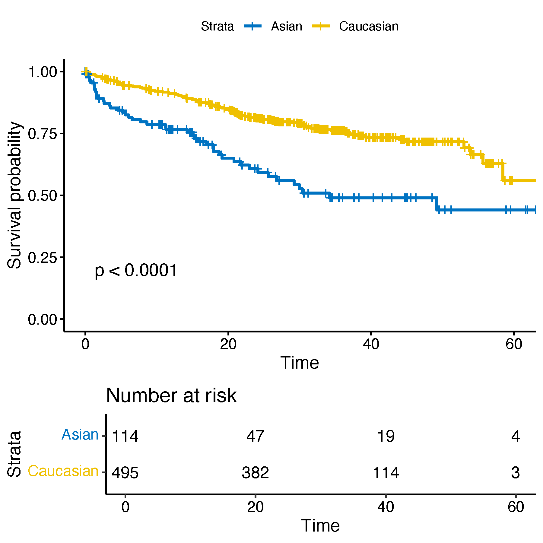
One potential explanation for this observation is that the HRD subtype is more prevalent among White patients, and this group also tends to have relatively favorable clinical outcomes within this subtype. However, despite sharing the HRD classification, Asian patients consistently exhibited worse prognosis, suggesting that molecular subtype alone may not fully account for outcome variability across populations.
When interpreted alongside the immune activation signatures observed in Asian HRD samples, this raises important biological questions. It is possible that the upregulated immune response represents a dysfunctional or exhausted state, which fails to confer clinical benefit. Alternatively, immune activation could reflect compensatory responses to a more aggressive or treatment-resistant disease course. These findings highlight the existence of ancestry-specific transcriptomic and prognostic heterogeneity within molecular subtypes, and underscore the need for stratified approaches when evaluating treatment strategies in diverse patient populations.
24.2 Mutational differences
To specifically investigate novel or population-enriched mutational patterns, we excluded samples harboring well-characterized structural alterations known to act as dominant drivers, and restricted our analysis to a curated panel of recurrently mutated genes in MM (PMID: 29884741).
Given that point mutations are not regarded as primary drivers in MM pathogenesis, we performed frequency-based comparisons only for selected somatic variants. Details are as follows:
pkgs <- c("fs", "futile.logger", "stringr", "jhtools", "glue", "tidyverse",
          "dplyr", "readxl", "ggplot2")
for (pkg in pkgs){
  suppressPackageStartupMessages(library(pkg, character.only = T))
}

workdir <- "/cluster/home/yjliu_jh/projects/mm/output/bar"
setwd(workdir)

genes <- c("KRAS", "NRAS", "DIS3", "FAM46C", "BRAF", "TP53", "HUWE1", "TRAF3", "ATM", "EGR1", "HIST1H1E", "DUSP2", "FGFR3",
           "PRKD2", "UBR5", "CYLD", "MAX", "IRF4", "ZNF292", "ACTG1", "KLHL6", "KMT2C", "SP140", "ARID1A", "CCND1", "CREBBP",
           "PTPN11", "KMT2B", "LTB", "ATRX", "TRAF2", "NF1", "EP300", "SETD2", "TET2", "RFTN1", "DNMT3A", "PRDM1", "RB1",
           "SAMHD1", "KDM5C", "SF3B1", "KDM6A", "NFKBIA", "XBP1", "ARID2", "NCOR1", "RASA2", "TGDS", "FUBP1", "MAF", "CDKN1B",
           "MAN2C1", "NFKB2", "ABCF1", "MAML2", "CDKN2C", "MAFB", "C8orf34", "ZFP36L1", "IDH1", "PIK3CA", "IDH2")

merged_sinfo <- read_rds("~/projects/mm/docs/meta/sampleinfo/sampleinfo_jilin_commpass.rds")

# commpass----------------------------------------------------------------------
commpass_wgs_fn <- "/cluster/home/jhuang/projects/mm/analysis/commpass/human/wgs/mutations/summary/commpass/41588_2024_1853_MOESM5_ESM_hg38.txt"
commpass_wgs <- read_tsv(commpass_wgs_fn) %>%
  dplyr::select(sample_id, GENE, Chromosome, Start_Position, End_Position, REF, ALT, EFFECT) %>%
  dplyr::rename(Hugo_Symbol = GENE, Reference_Allele = REF, Tumor_Seq_Allele2 = ALT, Variant_Classification = EFFECT) %>%
  dplyr::mutate(Variant_Classification = str_replace_all(Variant_Classification, c("missense_variant" = "Missense_Mutation", "stop_gained" = "Nonsense_Mutation",
                                                                                   "frame" = "Frame", "splice" = "Splice", "stop" = "Stop", "start" = "Start")))
kp_samples <- merged_sinfo$sample_id[merged_sinfo$subtypes %notin% c("CD_no_IgH", "CD1", "CD2", "MAF", "MS")]
commpass_wgs_fil <- commpass_wgs[commpass_wgs$sample_id %in% kp_samples, ]

commpass_wgs_mut <- commpass_wgs_fil %>%
  dplyr::filter(grepl("Missense_Mutation|Nonsense_Mutation|Frame", Variant_Classification)) %>%
  dplyr::select(sample_id, Hugo_Symbol) %>% distinct() %>%
  group_by(Hugo_Symbol) %>% dplyr::summarise(mutated_samples = n()) %>%
  dplyr::mutate(freq = (mutated_samples/length(unique(commpass_wgs_fil$sample_id)))*100)


# jilin-------------------------------------------------------------------------
jilin_mut_fn <- "/cluster/home/jhuang/projects/mm/analysis/meta/human/mutations/jilin_rna_wgs.rds"
jilin_mut <- read_rds(jilin_mut_fn) %>%
  select(sample_id, Hugo_Symbol, Chromosome, Start_Position, End_Position, Reference_Allele, Tumor_Seq_Allele2, Variant_Classification) %>%
  distinct()
jilin_mut <- jilin_mut[jilin_mut$sample_id %in% kp_samples, ]
jilin_mut_fil <- jilin_mut %>%
  dplyr::filter(grepl("Missense_Mutation|Nonsense_Mutation|Frame", Variant_Classification)) %>%
  select(sample_id, Hugo_Symbol) %>% distinct() %>%
  group_by(Hugo_Symbol) %>% summarise(mutated_samples = n()) %>%
  mutate(freq = (mutated_samples/length(unique(jilin_mut$sample_id)))*100)

gene_freq <- jilin_mut_fil %>%
  left_join(commpass_wgs_mut, by = "Hugo_Symbol", suffix = c(".jilin", ".cmps")) %>%
  dplyr::filter(!is.na(freq.cmps)) %>%
  dplyr::filter(Hugo_Symbol %in% genes) %>%
  mutate(fold = freq.jilin/freq.cmps) %>%
  arrange(desc(freq.jilin))

# plot--------------------------------------------------------------------------
pdf("genefreq_jilin_cmps_fil.pdf")
gene_freq <- gene_freq %>% arrange(freq.jilin)
max_freq <- max(c(gene_freq$freq.jilin, gene_freq$freq.cmps)) %>% round(digits = 0)
par(mar = c(5, 8, 4, 8) + 0.1)
barplot(gene_freq$freq.jilin, names.arg = gene_freq$Hugo_Symbol,
        horiz = TRUE, col = "#4e70bc", border = NA,
        xlim = c(-max_freq, max_freq),
        las = 1, main = "Alteration frequency (%)",
        cex.names = 0.5, xlab = "", axes = FALSE)
barplot(-gene_freq$freq.cmps,
        horiz = TRUE, col = "#ae2318", border = NA,
        axes = FALSE, add = TRUE)
axis(1, at = seq(-max_freq, max_freq, length.out = 5),
     labels = abs(seq(-max_freq, max_freq, length.out = 5)))
mtext("Commpass", side = 1, line = 3, at = -max_freq/2)
mtext("Jilin", side = 1, line = 3, at = max_freq/2)
dev.off()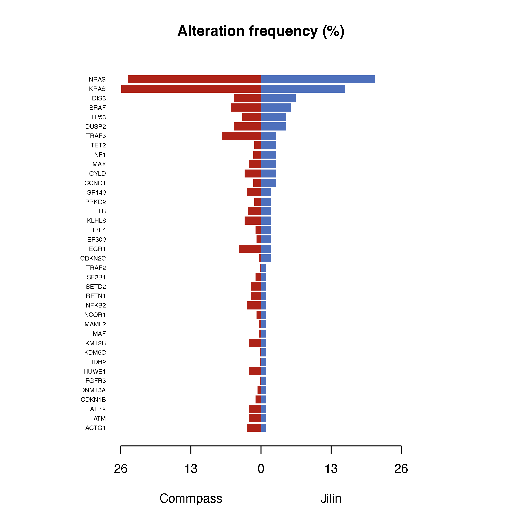
Consistent with prior reports suggesting population-level differences in somatic mutation burden, we observed a generally lower mutation frequency across several canonical driver genes in the Jilin cohort compared to the CoMMpass dataset. This finding may reflect differences in underlying mutational processes, selection pressures, or disease evolution between populations. Notably, mutations in CCND1, NF1, and TET2 were more frequently observed in the Jilin cohort. Increased CCND1 mutations may indicate a compensatory mechanism in cases lacking canonical CCND1 translocations, suggesting alternative routes to dysregulated cell cycle progression.